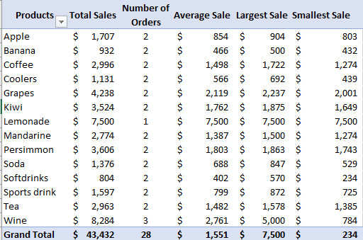
You will always find Excel either summarizing your data by adding the values together (SUM) or Counting the number of items. Nobody is stopping you from changing the type of calculation that your work demands to include averages, maximum, minimum, standard deviation and others.
Change the calculation from the Value Field settings.
- Add a column to your PivotTable by dragging a field from the list to the Columns section (as usual)
- Excel will make a new column using either the Sum or Count calculation depending on the source values.
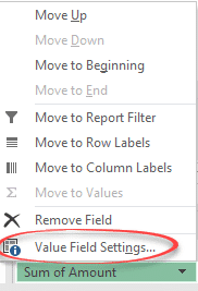
- Click on the selector next to the new column item and choose Value Field Settings …
- Summarize value field by … and choose the calculation you want. We’ve chosen ‘Min’ or minimum.

- If necessary, click ‘Number Format’ to change the way the values look.
Change an existing PivotTable field
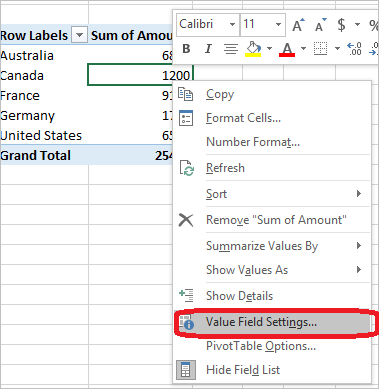
To change an existing field / column use the steps above or access the Value Field settings by right-clicking on any cell in the column.
Summarize / Calculation options
- Sum
- Count
- Average – mean
- Max – maximum / highest value
- Min – minimum / lowest value
- Product – multiplies all the values together.
- Count Numbers – counts only if the value is numeric. Blank, empty, text or error cells are not counted.
Standard Deviation and Variance
The last four options help to show the amount of variance or deviation between the values. The higher the Standard Deviation or Variance, the wider spread of the source values.
- StdDev – Standard Deviation, same as function S
- StdDevp – same as function P
- Var – Variance, same as function VAR.S
- Varp – same as function VAR.P