Making your first PivotTable can be scary so here’s a quick ‘How to’ to get you started and past the scary bit.
It’s a PivotTable starter article for anyone who hasn’t dived into PivotTables already and before we start with the tricks and tips for this important part of Excel.
Start with a list like this, a simple Excel worksheet.

PivotTables and PivotCharts can summarize lists in many different ways.
PivotTable Cheating
Modern Excel’s have a quick way to make a PivotTable ‘Recommended PivotTables’. Select your list then choose from the Insert tab.

Excel will try to figure out what PivotTable might be appropriate. It doesn’t always work out very well but it’s better than nothing.
It’s a quick way to start and very handy once you understand PivotTables.
We’ve seen many people get messed up by using Recommended PivotTables then trying to edit one to suit their needs.
We strong suggest you make some PivotTables yourself to grasp the basics. Then use Recommended PivotTables as a quick starter.
Make a PivotTable
Once you have your data ready, make a PivotTable the ‘old-fashioned way’.
- Click on any cell inside the your list.
- Go to Insert | Pivot Table from the Tables group.

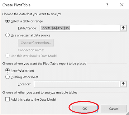
The Create PivotTable box appears. You can see that Excel has selected the data range for you, but make sure it’s guessed right. If you’ll be adding more data later, you might prefer to define a named range or a table.
Excel picks the default ‘New Worksheet’ as the place for the PivotTable report to be added.

Simply click OK.
Design a PivotTable
This is the step which confuses many people. Nothing seems to appear, just a strange set of mysterious message boxes. Never fear, Office Watch is here ….
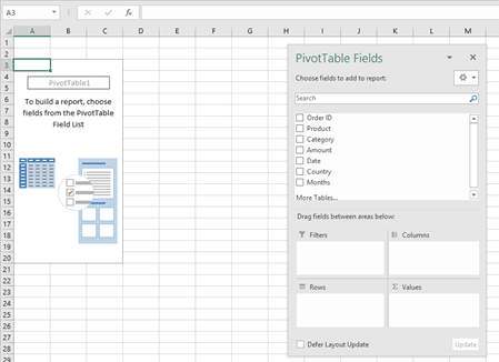
First thing, you will notice is a blank pivot table on the left side of your spreadsheet.

Look for the PivotTable Fields box on the right side of the worksheet. In case the Field (or Column) List is not displayed on the screen, go to Analyze tab and make sure the Field list is highlighted in the Show Tab.

Now that we have inserted the blank PivotTable let’s see how to add stuff to it.
Dragging fields
Start building your first PivotTable by adding list fields/columns (listed at the top) to the areas at the bottom: Rows, Values, Columns and Filters.
For a beginners PivotTable, just use Rows and Values – ignore the other two for the moment.
Microsoft’s preferred way is drag and drop the fields from the Field List to the PivotTable areas.
For example – You want to know the amount of each product exported, just drag the following fields to the different areas accordingly to filter the data.
- ‘Product’ field to the Rows
- ‘Amount’ field to the Values area.
The PivotTable panel looks like this.

Here’s your first Pivot Table. Isn’t it cool?

Pretty PivotTables and PivotCharts
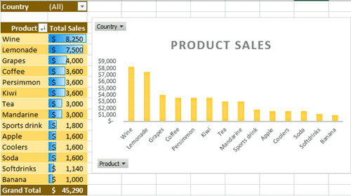
The basic PivotTable looks quite boring but add some formatting and a chart to make it look quite smart.

Just the beginning
That’s a mere first glimpse at what PivotTables can do. In upcoming Office Watch articles and in Office for Mere Mortals we’ll look at all the enhancements possible to this simple starter.
PivotTables can be sorted, like the example above to show ‘smallest to largest’ sales.
Filtering is possible, to see only part of a long list – see the ‘Country’ selector above. In fact, there’s many different ways to filter a PivotTable.
You’re not limited to adding up / Sum of totals. There are options to Count, Average and other more complex functions.
There’s some formatting necessary like changing the values to currency.
As we’ve already shown, many different PivotTables can be made from the one list.

Those somewhat clumsy headings like ‘Sum of Amount’ can be easily renamed.
PivotCharts can be made from PivotTables either directly or with a PivotTable as well.
PivotTables are automatically updated as the source list grows or is changed.