There are many situations where you need to split up text into separate columns. Names, phone numbers, dates, addresses and lot’s more can be managed with Excel’s Text to Columns,
Text to Columns allows you take data from one column, and split it out into multiple columns. This can be used to split full names or addresses up into separate columns, pull part of the data from one column out into a separate column, or myriad other uses.
First we’d like to warn about a big, enormous trap in Text to Columns …
Warning – overwrites existing data
For reasons passing understanding, normal computing practice and plain commonsense, Text to Columns will overwrite the source column! Here’s a very simple column of text that needs splitting into town names and state in different columns.
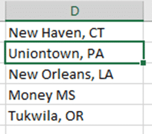
Run it through Text to Columns with a comma separator and this is the result.
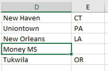
See that Column D has been replaced with the first column of the split text. Ouch. That’s bad if something went wrong, which it did in this example because one of the locations didn’t have a separating comma.
Happily, Undo will reverse Text to Columns but it’s normal computing practice to keep the source data intact … just in case.
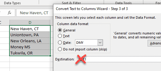
At step 3 of the Text to Columns wizard, always change the Destination to another column, probably the next to the right. In this case, change $D$1 to $E$1.
Delimited Text – Splitting up Names
We’ll start with a simple one, splitting full names up into given name and surname columns.
First, select the data you want to split, and go to Data | Data Tools | Text to Columns.
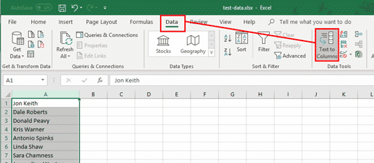
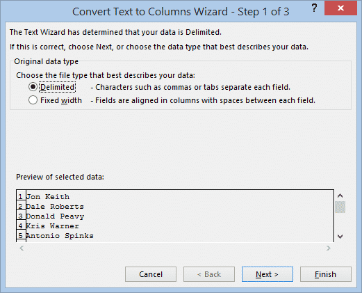
The first page of the Convert Text to Columns Wizard is where you specify what kind of data you are splitting. We have words with spaces between them, so we choose Delimited.
Fixed width would be used if you wanted to split out a certain number of characters from each field. We will look at an example of this later.
The second page of the wizard is also about the data that you are splitting, and is where you give more information about the format of that data.
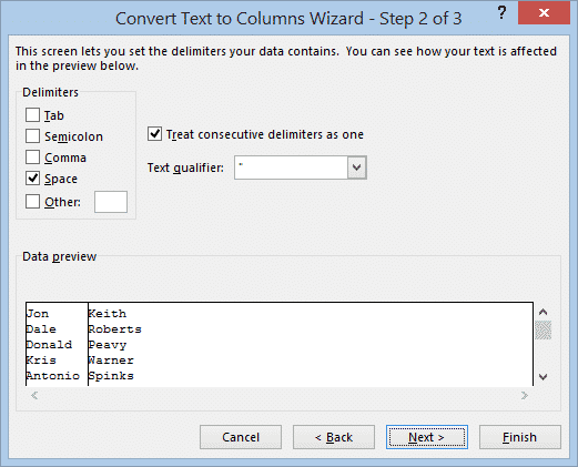
Our data has a space between the words we want to separate, so we tick Space. If you think there may be more than one space anywhere, it is a good idea to also tick “Treat consecutive delimiters as one”. Otherwise the extra space will be treated as another value and you will get a blank cell, with the surname thrown across into a third column.
The preview box at the bottom shows how the data will be split, so scan down that to check that everything looks all right. When you’re happy with it, click Next.
The third page of the wizard is where you specify what happens to the data after the conversion.
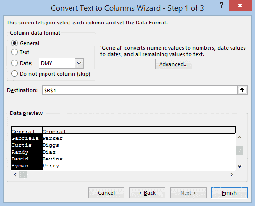
As we’ve said already, the important part here is the Destination field. If you don’t change this, the converted data will overwrite the existing data, which may not be what you want. I want to keep the original column and place the new format data next to it, so I have chosen cell B1.
Show your work
Note that if you need to look more closely and see the fields that the wizard is covering up to work out where to put the data, you can click the arrow button at the right of the Destination field to hide most of the wizard. Click the arrow again to show the full wizard again.
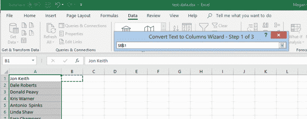
When we’re happy with our settings, click Finish, and our names will be split into two columns.
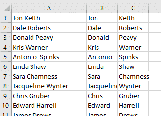
This is a good example of splitting two words into separate cells. However, in practice, Flash Fill might be a better choice. Flash Fill can be ‘trained’ to cope with common name variations like middle names or initials, surname prefixes like ‘Van’ etc.
Fixed Width – Separating text
For this example we have a list of numbers that are actually phone numbers entered without any formatting.
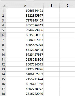
We want to separate out the three-digit area code from the phone numbers, so we again select the data and click on the Text to Columns button.
This time, however, as it is always the same number of characters that we want separated, we select the Fixed Width option.
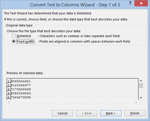
This time when we get to the second page, we can see that there is a ruler above the data preview. The numbers on the ruler represent the number of characters in the data.
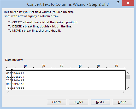
As we want to separate out the first three digits of the numbers, we click after the third digit, and a line will appear to mark the break point. If we put the line in the wrong place, we just click and drag it to move it. If we put in an extra line that we don’t need, just double-click on it to remove it.
Then we click Next to go on to the third page again.
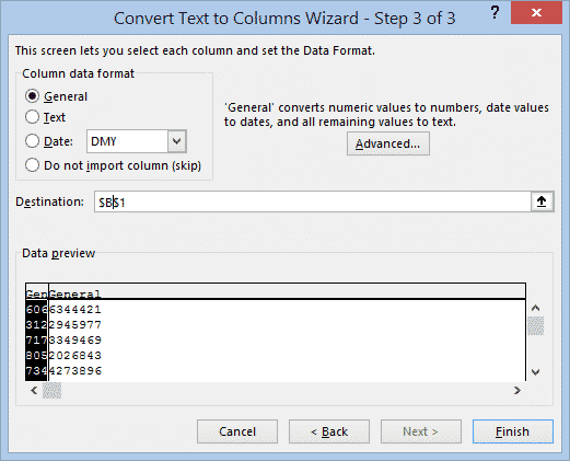
Set the Destination cell of where we want our separated data to start, and click Finish. We now have the numbers split up into area codes and phone numbers.

Fixed Width – separating area code
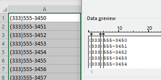
A more common situation is separating a phone area code in brackets from the main number. For example (303)555-1234 into columns for area code and number.
That’s possible with the Fixed Width option and putting the brackets into their own columns with breaks like this.
Two ways to handle unwanted columns
There are two ways to handle the unwanted columns – the official way and the cautious choice.
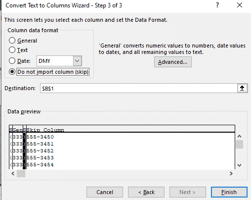
The official choice is ‘Do not import (skip)’ which is great if you’re absolutely sure the Text to Columns split works 100% of the time. In other words that the data is consistent.
The more cautious choice is to let the unwanted columns go through into new columns. Then you can check if the split text is correctly done. You’ll end up with columns like this:
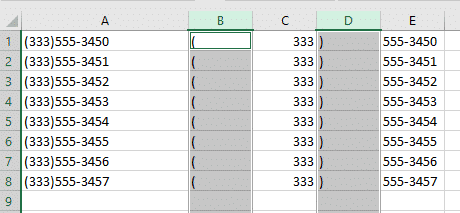
Delete the columns with brackets (B and D) and you’re good to go.
Advanced Settings
These are just a couple of simple examples that don’t come near to exploring the full range of things that can be done with this feature. We also haven’t looked at some of the more advanced settings in the wizard that would be used for more complex operations, but we’ll just touch on them briefly here.
Text Qualifier
If you are using delimited data the second page of the wizard has a field called Text Qualifier, which has three options: none, a single quote mark, or a double quote mark.
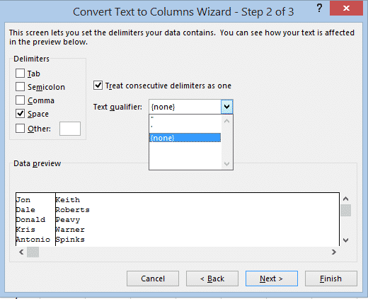
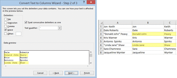
This is used if your data contains instances of the delimiter character within the text itself, that needs to be treated as regular text and not as a place to split the data. For example, with our name data, if some of the people had middle names, and we didn’t want a separate middle name column, but just wanted these to go in the Given Name column with the first name, we would need to enclose both of the given names in the qualifier character, which tells Excel to ignore any spaces within that data.
So if we select the double quote mark (“) as our text qualifier, our input data would need to look like this:
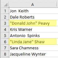
Which would cause both names within the quote marks to go into the given name column.
Column Data Format
This section on the third page of the wizard allows you to set the format for each of the columns that will be created. Click on each of the columns in the preview and select a format for it. If one of the columns is to hold dates, also select the date format.
Skip or do not import column
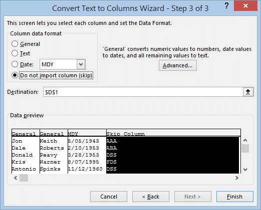
If part of the data is not required, you can select “Do not import column” and no column will be created for that data.
Below is an example where the original data include people’s names and dates of birth, as wall as a code, all in the one cell. We want to split up the names and dates of birth, and discard the codes.
Recognize numeric data
The Advanced button on the third page of the wizard contains settings for how to recognize numeric values in the source data – whether decimals and thousands are indicated by a comma or a dot, and whether a dash after a number should be regarded as a negative number.
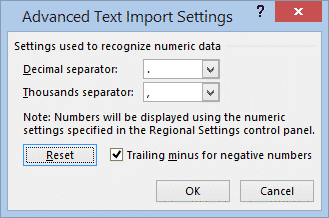
The decimal and thousand settings will default to the settings of the Regional Settings of your computer, and generally would not need to be changed unless you are importing data from another country that uses a different number format.