The venerable SUM() function in Excel is simple, really too simple. It just adds up a range of cells with no way to filter or limit what’s included. SumIF selects what to add-up from a longer list.
SumIf sometimes confuses people because they, understandably, expect the range to be SUMmed to come first followed by the condition. After all, most functions based on others start with the same parameter order as it’s ancestors then extend the features for more options at the end..
With SumIF the conditions come first and the values to be added up are last.
SUMIF(<range of filter criteria>, <criteria to search for>, <range to sum>)
Range of filter criteria . It’s the range of cells that you want filtered. The range can be numbers, names, arrays or dates. Microsoft calls this just ‘range’ which just add to the confusion.
Criteria to search for. This can be a single value to match eg “64” “Dopey” “Tuesday” or a cell reference to a value. Or a short IF filter like <64 for values below 64.
Any text criteria or any criteria that includes logical or mathematical symbols must be enclosed in double quotation marks (“). If the criteria is numeric, double quotation marks are not required.
You can use the wildcard characters—the question mark (?) and asterisk (*)—as the criteria argument. A question mark matches any single character; an asterisk matches any sequence of characters. If you want to find an actual question mark or asterisk, type a tilde (~) preceding the character.
sum_range The actual cells to add up after filtering. If you want to SUM the same range as you’re filtering (e.g. Sales over 1,000) then this parameter isn’t needed. Excel will assume you mean to filter and SUM the same range.
Very commonly, the search range is different from the SUM range. Most likely matching columns of a list (e.g Sales for a single name). That’s when you add the third parameter to tell which range to add up.
SumIF in action
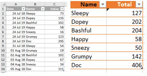
A simple example of SumIF at work with a simple table. Adding up the values for each dwarf is a perfect job for SUMIF.
Each of the Total (right) are made with the formula:
=SUMIF($B$2:$B$14,E2,$C$2:$C$14)
Here’s how it’s done with =SUMIF(Dwarves[Name],E2,Dwarves[Value]).
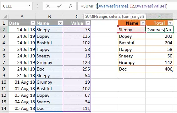
We’ve made a separate table with the names of the short seven in one column. The neighboring column has the SUMIF:
Search Range is Dwarves[Name], the list of names in the original table.
Criteria is the next-left cell with the current dwarf’s name.
Sum Range is the list of values in the original table.
In this example, we’ve typed the list of individual dwarfs but in the real world it’s faster and more adaptable to make the unique list based on the original.