Previously we talked about How to add a Drop-down List in Word, but you can also work more efficiently in Excel worksheets by making use of drop-down or pull-down lists. We will show you how to use Microsoft Excel’s data validation function to create useful lists within your spreadsheets. How to avoid the trap that lies waiting for the unwary who follow Microsoft’s ‘simple’ instructions.
It is especially useful when you need to do data entry work. The names, products etc are kept consistent with no typing mistakes.
Microsoft recommends having your pull-down list entries within an Excel Table, you can do this by simply selecting the cells/range of your text and pressing Ctrl + T | OK. You can also tick the ‘my table has headers box’ if you have a header already, here we’ve used Stage Names.

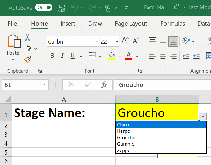
Now, select the cell that you want the drop-box to appear. For this example, we will be inputting the drop-box into C1.

Next, go to the Data | Data Validation
Within the Data Validation Settings tab, select List from the Allow drop-down.

Select the source box and then select your list range from the table. For our example, we put ours in a worksheet called Names, and the range of cells are $A$2:$A$6. Sounds easy but it’s a trap!
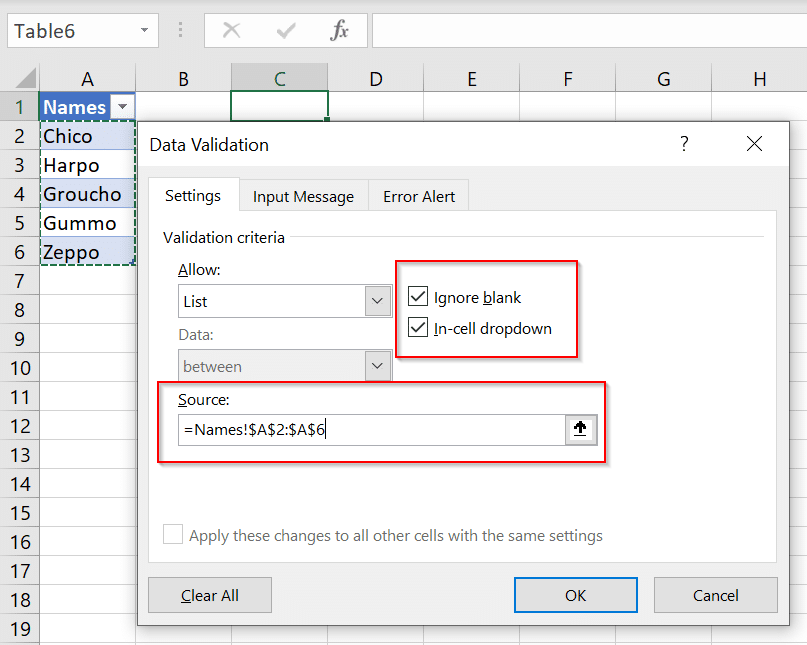
Excel inserts a fixed range of cells for the pull-down list. If you change the number of items in the table list (add/remove names) Excel will still only show the cells referenced.
What you need is a variable list which will expand and contract automatically.
Using an Excel Table for the pull-down list
The smarties among you probably think that’s easy, just reference the table not the cells. For example use =MarxBrothers[Stage Name] instead of $A$2:$A$6 . That should work. Alas, that doesn’t work because Excel Data Validation doesn’t accept a dynamic spilled array. You’re welcome to try but Excel gets all confused like this:

There’s a workaround that should not work but does.
Excel won’t accept a table reference directly, but will accept a named range linked to a table reference. In other words, disguise the table ref with a different name and Excel will stop complaining.
Go to Formula | Define Name and make a new named range. In Refers to: select the table column (no header) and Excel will insert the table and column named reference.

Now go to the Data Validation setup and use the named range as the Source:

Add or remove entries
Now let’s put the Excel Table feature we mentioned earlier into action.
When your data is in a table and it’s properly reference in the pull-down list, once you add or remove anything from the list, anything based on the table that’s included in the drop-down list will automatically update. So you won’t have to worry about fiddling around with updating the drop-down list, just update the table.
Advanced users can link to other data sources to populate the pull-down list. For example, link to an external database for a list of current staff members, customers or products. Use PowerQuery to import the latest data and load into a table.

We have removed Zeppo from the list, by completely deleting the row. Note, if you only delete the entry from the cell, it could still leave a blank space within your drop-down list.

Hide the source table
Now you can easily hide the source cells or table column A by selecting Hide.

Use Another Sheet
Another option, rather than hiding columns within your worksheet, is to place the data entries in a separate sheet/tab to your pull-down list.
Here we have placed the entries into an Excel table in a sheet/tab called Data.

Now we have the option to completely hide the sheet. Right click on the tab and select Hide. (To unhide the sheet, simply right-click your original sheet, select unhide and select the sheet).

From here, we can select the entries from the drop-down box in our original spreadsheet with the source hidden away.

Want more? Using Unique() to make an Excel drop-down list
How to add a Drop Down List in Word