The last two weeks we’ve been looking at getting current information from the internet into a worksheet, like currency exchange rates and stock prices.
Now let’s look at how to take that information and use it in your worksheets.
For this article, we’ll be using Excel 2016 for Windows because it has ‘Get & Transform’, formerly known as PowerQuery. Excel 2013 has PowerQuery as a free add-on from here.
PowerQuery/Get & Transform makes getting data and using it in Excel considerably easier than in earlier versions. The same thing is possible in earlier versions of Excel but you’ll have to either add some VBA code or remember to manually re-sort the imported list after each refresh.
First, let’s look at the basics of grabbing a value from a list. Then we’ll show how to ‘massage’ the internet data so it’s possible and easier to use in Excel.
The aim is to take a long list of regularly updated value. In this case, the current exchange rates:

And turn it into a calculation sheet that you can use for the values and currencies of your choice.

Enter the amount on the left then the currency to see the equivalent in US dollars. The fourth column is the full currency name, to reassure you that the three letter code selected is the right one.
VLOOKUP()
The key to all this magic is the VLOOKUP() function that’s been in Excel for many years.
VLOOKUP searches a worksheet list for a match with the value you specify, if it finds a match, it will return a cell to the right of the matching cell.
The official syntax is:
VLOOKUP (lookup_value, table_array, col_index_num, [range_lookup])
Lookup_value – is the value you want to find in the source list.
Table_array – the range of cells in the lookup list. This includes the column to search and the column you want returned as the result. In the above source list the table_array is columns A, B and C.
The first column of the table_array is the column Vlookup() will search down to find a match.
Col_index_num – which column to use for the result value. The second column to the right (Col B, exchange rate) is 2, third column (Col C, targetname) is 3 and so on.
Range_lookup – changes the way VLOOKUP searches the list. It doesn’t worry us in this example but, for future reference:
- TRUE (the default) searches for the closest match to the lookup_value and assumes the list is sorted.
- FALSE looks for an exact match in the searched column. Using VLOOKUP() with an unsorted list is theoretically possible but the results are ‘erratic’ to put it mildly. Far better to stick with a sorted list.
Here’s VLOOKUP() in action:

=VLOOKUP(B2,'USD rates'!A:C,2)
It gets the exchange rate for the currency code in column B ( = AUD), from the table in the ‘USD Rates’ worksheet (columns A, B and C only).

and returns the value from the second column to the right (= 1.3193879).
Setting up your list for VLOOKUP()
The secret to VLOOKUP() is the setup of the table it searches.
- The column to lookup is the first (left most) column in the table. It doesn’t have to be column A but it does have to be the first column on the left of the target range.
- That search column should be sorted (alphabetical or numerical). VLOOKUP works best and faster this way.
- The other columns in the table, the ones you’ll get values from, must be to the right of the searched column. In other words, the results column must be a ‘higher’ column than the searched column.
That’s where Get & Transform / PowerQuery comes into it’s own. It can easily create a table in the form that VLOOKUP needs. This was possible before PowerQuery but more cumbersome.
Let’s look at the exchange rate data feed we’ve already made and arrange it into a VLOOKUP() friendly fashion. Choose the data table and from the Query tab choose Edit to open the Query Editor.

As you can see, the three data columns we need (targetCurrency, targetName and exchangeRate) are already in the correct order (with targetCurrency on left). If they aren’t, it’s easy to change see ‘Position of columns’ below.
Sorting
Sorting is an amazingly long standing problem for external data feeds in Excel. Until PowerQuery, there was no simple way to re-order a data list and make that sort stick after the data is refreshed. You needed VBA code to force a resort after the incoming data was refreshed.
The correct sort order is necessary to make VLOOKUP() work reliably.
Microsoft didn’t think that was a problem because they arrogantly assumed you had control over the sorting order of the incoming data. That wasn’t always the case. You could either change the SQL statement to force a sort (ORDER AS) or ask the data supplier to change the sort order to suit your needs. But that’s not the case with public data feeds, so the sorting problem was an unnecessary stumbling block for Excel users.
Get & Transform / PowerQuery (finally) fixed that by including a sort option in the query.
It’s so simple and obvious, it’s almost embarrassing to explain it. Sorting works the same as a standard Excel worksheet. Click on the arrow in the column heading and choose Sort Ascending.
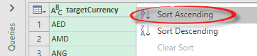
That’s it! Any time the data feed is updated, the query result will be automatically sorted into that order (unlike the same setting in a normal Excel worksheet).
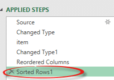
The sorting shows up in the ‘Applied Steps’ of the query.
Position of columns
Rearranging the columns in a query is sometimes necessary to make VLOOKUP() work with the searched column on the left and the other values to the right.
It’s not strictly necessary, but easier to manage, if the columns you want are the left-most ones in the list. Moving columns is officially done by right-clicking on the column heading and choosing Move | Left.

But it’s probably easier to ‘drag and drop’ the column header across to the position you want.
It’s also possible to select multiple columns (hold down Ctrl and click on headers) then either use Move | Left or drag ‘n drop.
However, you do it, the columns end up on the left side of the data list.
