From Excel 2010, Microsoft added Slicers to Excel’s PivotTables. From the hype, Slicers sound like some complex Excel feature but they’re really a more useable, friendly and showy way to do something already in Excel – Filtering.
For me it’s more of a visual filter and a collaborative tool that can help you figure out what items are selected within a PivotTable. Yes, they are always associated with PivotTable.
On the left is the PivotTable. On the right are two Slicers with selections to filter what’s shown in the PivotTable.

The selected product buttons choose what’s shown on the PivotTable.
All amounts are displayed but the Slicer buttons have different colors whether the current PivotTable includes those values or not. You could also filter the PivotTable by the second slicer.
Using a Slicer, you can filter your PivotTable data in a more visually interesting and dynamic way. Create and copy a slicer associated with the PivotTable. Even better use a single slicer to filter multiple PivotTables.
Inserting a Slicer in an existing PivotTable
Take any PivotTable that you’ve created. Navigate to Options | Analyze | Insert Slicer
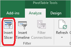
Select ‘Category’ and ‘Date’ check box and click Ok

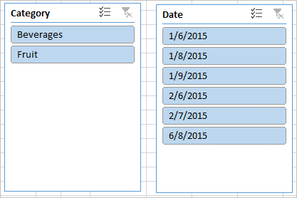
Cool! Now that’s your fancy little slicers below. You got a Category slicer and a Date slicer. Likewise, you can now play around your data. Try to slice and dice your data as you like it.
For example, click on Beverages in the ‘Category filter’ and a Date (I have selected 6/8/2015) – that would give you what beverage was exported on that date.
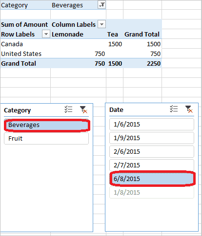
When you choose the ‘Category’ as ‘Beverages’ the report filter also changes to ‘Beverages’