Protecting an important Excel worksheet from careless editing, or allowing only specific cells to be modified is all part of a powerful and highly flexible feature in Microsoft Excel known collectively as “Protect”. It’s been there for a long time but is little understood, so we’ll do our humble best to fix that.
The idea behind “Protect” is that many large spreadsheets are often filled with elements of differing levels of importance. It is a preventative measure against anyone from accidentally or deliberately changing, moving, or deleting important data within an Excel worksheet.
For example, imagine a spreadsheet with a large data entry area, some informative text on how to use the worksheet, and a few formula related to the data entry area. The formula will probably need to remain constant, as will the informative text, but the data entry fields around them will always need to be editable.
If you send the spreadsheet to other people you don’t want them changing the text and formulas – just change the data entry cells and view the results.
All this is done at the Review | Protect submenu provides options to “Protect Sheet”, “Protect Workbook”, “Allow Edit Ranges”, and “Unshare Workbook”.

LOCKING NEEDS PROTECTION
Each cell in a worksheet can be either locked or unlocked – that in itself means nothing until the worksheet is ‘Protected‘.
By default all cells are set as locked – see Home | Cells | Format | Format Cells… | Protection but that locking will only apply after you’ve gone to Review | Protect and applied protection to some part of the spreadsheet.
Keep this difference in mind – many people, including us will talk about ‘locking’ a worksheet when it’s really a two step process – lock then protect.
LOCKING AN ENTIRE WORKSHEET
Locking an entire worksheet from editing is one way of giving it a “read-only” status. This means that anyone who has access to the worksheet (including you) will not be able to edit any fields unless the worksheet is unlocked.
This could be useful if the spreadsheet in question formed a finalized set of budgetary figures. In this situation, you probably won’t want the worksheet to be modified by anyone including yourself. Any inadvertent changes to a document of this nature could have far-reaching consequences.
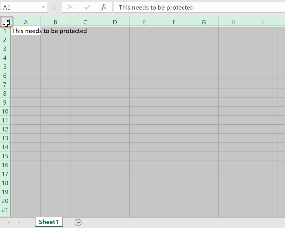
To begin locking the worksheet, select the entire worksheet by clicking the “Select All” button (the gray rectangle directly above the row number 1 and to the left of column letter A).
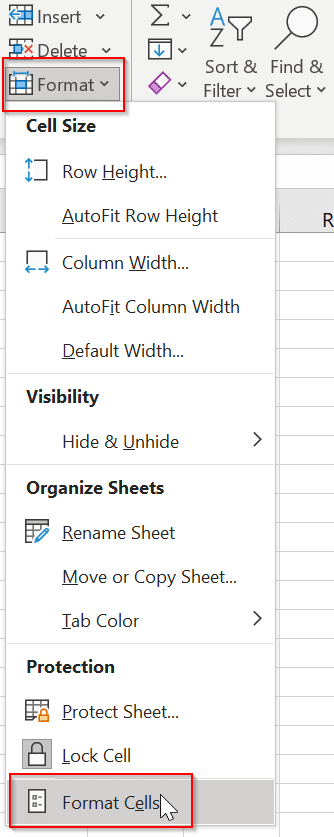
Then navigate to “Home | Cells | Format | Format Cells…” and select the “Protection” tab. Click on the “Locked” checkbox until a tick appears and then click “OK”.

This alone will not lock the cells for editing. In fact, you may have noticed that all cells are actually “locked” by default. The “locked” cell attribute will only take effect after protection is enabled. (as well as the “hidden” cell attribute)
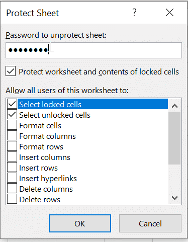
To enable protection, you must navigate to “Review | Protect | Protect Sheet”. In the “Protect Sheet” dialog box, ensure that the “Protect worksheet and contents of locked cells” checkbox is checked.

Now type a password that must be used to “unprotect” the worksheet. Choosing a password might not be necessary if you are only guarding against your own “accidental” changes. However, if you don’t supply a password, then any other user will be able to unprotect the sheet and change the protected elements.
Finally in the “Allow all users of this worksheet to” list, select the elements that you want users to be able to change before clicking “OK”.
OTHER LOCKING OPTIONS
By default, you are only able to “select locked cells” and “select unlocked cells” on a protected sheet. Other options include:
- Format cells
- Format columns
- Format rows
- Insert columns
- Insert rows
- Insert hyperlinks
- Delete columns
- Delete rows
- Sort
- Use AutoFilter
- Use PivotTable and PivotChart
- Edit objects
- Edit scenarios
When protection is no longer needed, the process is easily reversed by going to “Review | Protect | Unprotect Sheet”. If you initially set a password to protect the sheet, then you will be prompted for it. Otherwise, the sheet has been unlocked and editing is once again made possible.

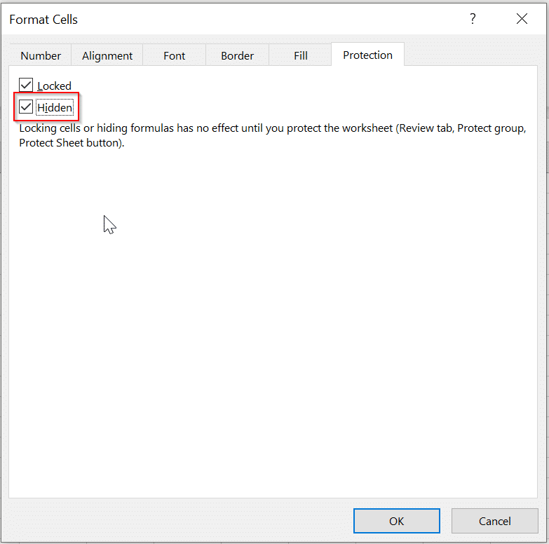
HIDDEN CELL ATTRIBUTE
We mentioned the “hidden” cell attribute above. Hold down the CTRL key and select any cells that contain formulae that you don’t want to be visible. Again, navigate to “Home | Cells | Format | Format Cells…” and on the “Protection” tab, click the “Hidden” checkbox until a tick appears. Now click “OK”.