How to lock certain cells in an Excel workbook and allow people to edit ranges of cells.
In part one we covered the basics, how locking works with protection to stop unwanted editing of your worksheets while leaving them visible.
Now we’ll cover some more, locking certain cells in a worksheet and allowing people to edit ranges of cells. Plus a quick note on ‘strong’ passwords that applies not only to Excel but anywhere you enter your password.
LOCK ONLY A FEW CELLS ON A WORKSHEET
Only locking a few cells on a worksheet can be achieved by a similar method. To start off, select the entire worksheet, navigate to “Home | Cells | Format | Format Cells” and click the “Protection” tab. Click the “Locked” checkbox until it is clear and click “OK”. This unlocks all of the cells in the worksheet.

Of course, you can do it the other way around. Select the cells to unlock and leave the rest in the default ‘locked’ mode.
If the “Cells” menu function is not available, parts of the worksheet may already be locked and protected. If this is the case, you will need to unprotect the worksheet by navigating to “Review | Protect | Unprotect Sheet”.

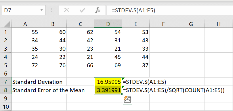
Now select a range of cells on the worksheet that you wish to lock (such as the all important formulae). This can be done cell by cell, or all at once if you wish.
Color change is helpful
Once they are selected, you can optionally change the “fill-color” of the cells in the toolbar to something that distinguishes them from the other cells. Yellow would do the trick, but you can choose whatever you want. Changing color makes no difference to Excel but helps us mere humans work out what cells are protected.
Making sure that these cells are still selected, navigate back to “Home | Cells | Format” and click the “Lock Cell” button under “Protection”. This will lock all of the selected cells.

LOCKING AND COLOR
The only reason we choose a different background color for these cells was to help users to easily distinguish between locked and unlocked cells. Surprisingly, there is no simple feature within Microsoft Excel that can be switched on to make this distinction.
Finally, navigate to “Review | Protect | Protect Sheet”, and select a password. The worksheet will now have some cells locked from editing and highlighted to distinguish them from the other unlocked cells. Double-clicking on a locked cell will also bring up a message box detailing its read-only status.

ALLOW SPECIFIC USERS TO EDIT RANGES
Another function in the “Protect” feature as a whole is to give specific users access to protected ranges of cells within a worksheet.
To begin with, select the range of cells you wish to share with a particular user. Then navigate to “Review | Protection | Allow Edit Ranges”, noting that this command is only available when the worksheet is not protected.
In the “Allow Edit Ranges” dialog box, click the “New” button. In the “Title” box, type a title for the range you’re granting access to, such as “Formulae Range” or more wistfully “Golf Driving Range”.
Since we had selected the range of cells the rule would act upon already, they will appear inside the “Refers to cells” box.
In the Range password box, type a password to access the range. Again, the password is optional. But if you don’t supply a password, any user will be able to edit the cells.

Now click on the “Permissions” button, and then click “Add” in the resulting dialog. Locate and select the user(s) to whom you wish to grant access. You can also Check Names first by entering the object names to select (click on the examples link for more info). If you want to select multiple users, hold down the CTRL key while you click the names.

Repeat the previous steps for each range and then click the “Protect Sheet” button within the “Allow Edit Ranges” dialog box.
Finally, in the “Protect Sheet” dialog box, make sure the “Protect worksheet and contents of locked cells” check box is selected. Then type a password for the worksheet, click “OK” and confirm the password. This will activate the selective protection, whereby only specific users are able to edit specific ranges of cells within the worksheet.

SELECTING A PASSWORD
A worksheet password is required to prevent other users from being able to edit your designated ranges. Excel passwords can be up to 255 letters, numbers, spaces, and symbols.
Make sure you choose a password you can remember, because if you lose the password, you cannot gain access to the protected elements on the worksheet.
Any password you use on your computer should be a “strong” one. But how do you know if what you’ve selected is a strong password?
The strongest passwords look like a random collection of uppercase, lowercase, digits and symbol characters. Preferably no characters are repeated, and the digits or symbols are not used as the first or last character.
Another rule of thumb is that strong passwords are at least seven characters long and do not contain characters that are consecutive such as “1234”, “abcd” or “qwerty”. Finally, a strong password does not contain complete names or words in any language, especially related to your name or username!