Gridlines are on every spreadsheet in Microsoft Excel workbooks. Did you know those grey lines can be colored to make them fancy, more obvious or more discreet? Let’s look at two ways you can make colored gridlines in Excel.
Here’s what it looks like with the pink, black and red in comparison to the default grey, quite a considerable difference.

Excel Gridline Color
By using a different gridline color, in comparison to the default light grey, this’ll make it easier to see on the screen due to the greater contrast between the background and colored gridlines.
Firstly, you’ll need to open your Excel workbook and go to File | Options | Advanced.
This will open the Excel Options window, now, scroll down until you see ‘Display options for this worksheet.’
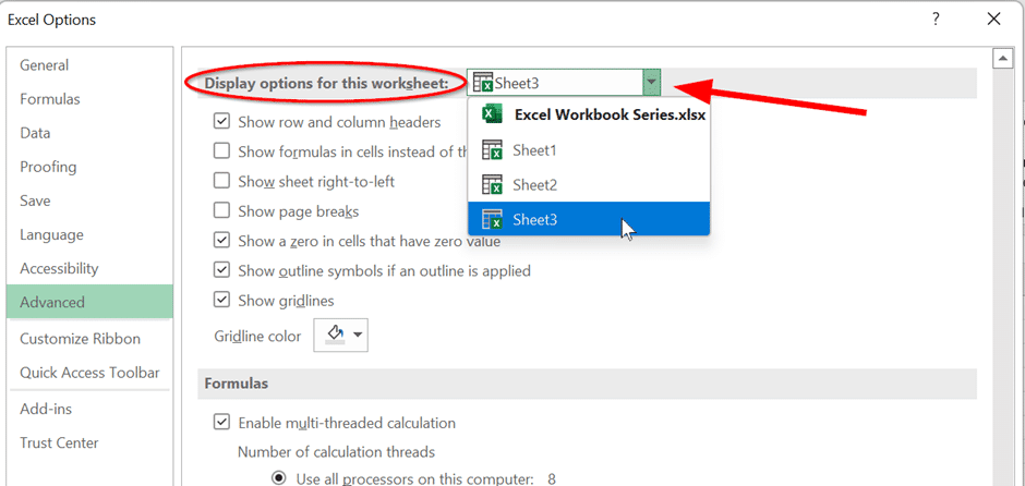
Choose to change the settings for the whole workbook or just one sheet. There is a drop-down box that will display the current worksheet selected. You can click and select an alternate worksheet if you wish.
We like to change the gridlines for selected sheets, so it’s easier to tell the difference between each tab. That’s really handy when the sheets are showing different views of the same data.
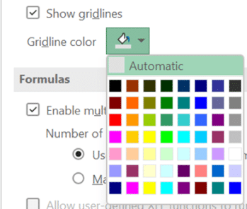
At the bottom of this section the Gridline color, followed by a paint tool where you can select a different color. Simply choose your preferred color, you might go with a darker color such as black, or a bright color such as pink. Either way, the choice is yours, so long as you go with a color that produces a good contrast.
Once you’ve selected OK in the bottom right corner, the changes will apply to your selected spreadsheet.
Apply a Border to cells
Another way to add more emphasise to your gridlines, is to apply a border to the entire sheet or part of a sheet. This is the more familiar way to color gridlines.
This changes the border settings for all or selected cells on the worksheet and will show up on printed versions of the sheet.
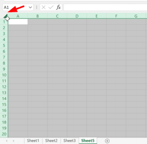
You’ll need to firstly select the entire worksheet or part sheet Select all using the keyboard shortcut Ctrl + A or clicking on the green triangle near A1.
Next, go to the Home | Cells | Format | Format Cells
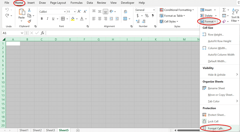
(Or just use the quick keyboard shortcut Ctrl + 1).
This will bring you straight to the Border Tab, where you can adjust the line style, color, and presets.
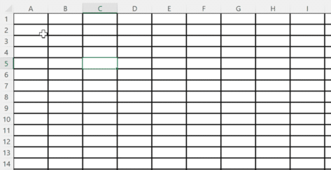
In our example we have chosen a thicker line, the color black, as well as presets in both the outline and inside.

It’ll provide you a preview of your changes prior to clicking on OK.
Of course, you can change the color and thickness to anything you like.
Once you’ve selected OK, the border style will be applied to your worksheet.
If you’re unhappy with the changes, just simply click Undo and it will revert to normal.
Flash Fill Magic in Excel
More powerful Excel Autofill using Series
Pound £ symbol in Word, Excel, PowerPoint and Outlook
Redacting Excel worksheet