An IF statement might sound like a complicated thing that programmers do, but it’s actually fairly easy to do in Excel. An IF statement basically puts something into a cell depending on certain conditions – if A is true, put X in this cell. You can even use what’s called a nested IF statement if you have multiple conditions that you want to meet.
To start with a simple example, let’s say we have a spreadsheet where we enter our expenses, but any expense over $100 needs to have an authorization number, so we want a note next to those expenses to remind us that we need to enter that number.
The Original IF statement
The basic format for an if statement is:
=IF(condition-to-be-met,what-to-insert-if-true,what-to-insert-if-false)
If that looks complicated, don’t worry, as Excel has a handy tool to fill all this in for you.
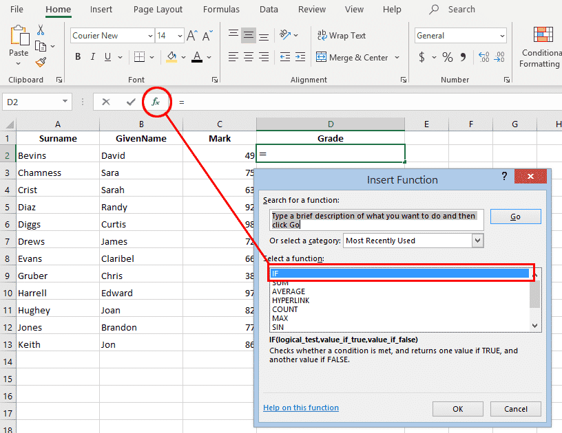
To create an IF statement, click in the cell where you want the result of the statement to appear (in our case, in the first cell next to the amount column), and click the Insert Function button.

Of course, you can just type =IF and Excel will offer prompts and reminders

But the Insert Function dialog helps you select the right function and shows a full dialog box to type in the right parameters.

The logical test is the condition that we want to have met. We are interested in if the amount in cell B2 is greater than 100, so we write:
B2>100
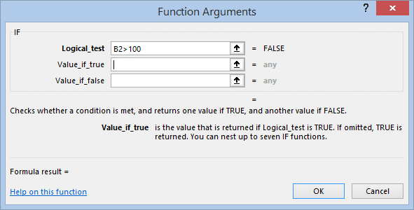
The full function arguments dialog is great for anyone new to a function or trying to fix a problem.
- The current result for a parameter appears to the right.
- The text explains what goes in the currently selected parameter.
- Click on the up arrow to briefly shrink the dialog and let you see or choose values from the worksheet.
- The current result from the function appears bottom left.
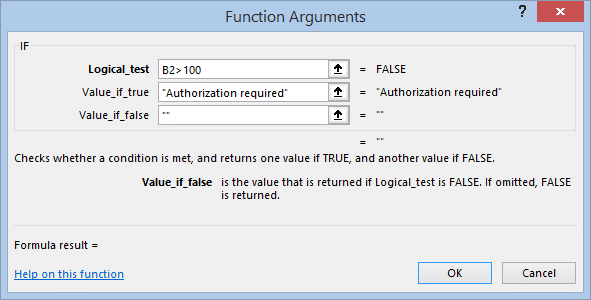
Now we need to specify what happens if the contents of cell B2 meet this condition. If we want text in the cell, we need to put quote marks around the text. So in the Value if True field, we type:
“Authorization required”

Now, we don’t want anything to appear in the cell next to amounts less than $100, but if we leave the Value if False field blank, Excel will enter the word FALSE in any of those cells. To have those fields remain blank, we need to enter quotation marks with nothing in between them in that field.
Click OK and we will see our function in the formula bar.

This function is still only applying to cell C2 though, so, just with any other formula we enter, we need to grab the bottom right corner of the cell and drag down to apply the formula to the whole column.

Now, as we fill our spreadsheet with expenses, anytime we enter an amount that is more than $100, the message “Authorization required” will appear next to it to remind us that we need to enter the authorization number, and make it easy for anyone auditing the expenses to check that authorization has been entered for any relevant expenses.

Nested IF statements for multiple conditions
If you have more complex conditions to meet, you can use nested IF statements. It’s not immediately obvious how to do this using the wizard we used above, but it can be done!
Let’s say we want to enter our students’ grades into a spreadsheet, and we have a grading system structured as follows:
0-49 = FAIL
50-69 = PASS
70-79 = CREDIT
80-89 = DISTINCTION
90-100 = HIGH DISTINCTION
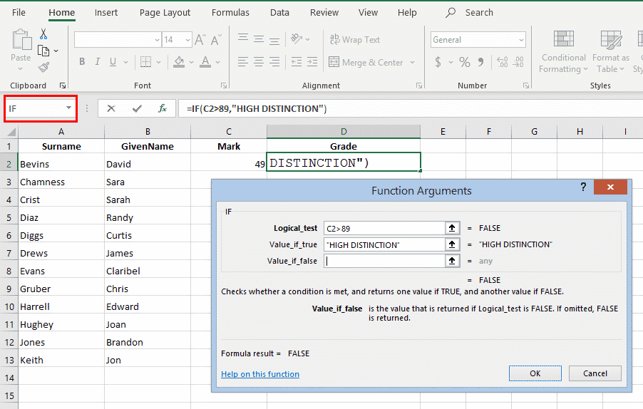
We will start out using our highest grade. If 90-100 scores receive a High Distinction, then we need to specify what happens for a score over 89. We start out as if this is our only condition. As above, we click the Insert Function button and select IF to open the Function Arguments dialog.
Now write our first condition (greater than 89) and the result if that is true (“HIGH DISTINCTION”), but don’t put anything in the Value if False field yet.

Now we click in the Value if False field, but instead of typing anything here, we then click on the Name box, which should still say IF.
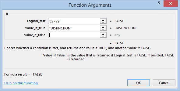
This will open a new blank Function Arguments dialog, where we enter the next condition and result – any score over 79 should receive a Distinction.
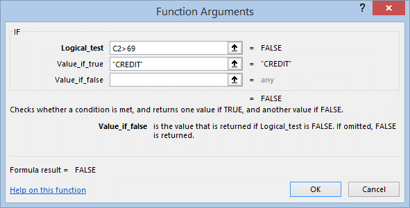
Then repeat the process for the Credit result.
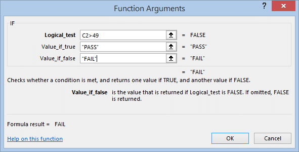
Then we do again with the Pass condition, but this time we don’t click back into the Name box. We only have one result left (Fail), and this is what happens when none of the above conditions are true, so we can put that last result into the Value if False field. If the student’s score is not over 49, they receive a fail.
As you are entering all this information, keep an eye on the formula bar to get an understanding of the structure that is being created. Each time you enter a new condition, a new set of parentheses is opened within the previous set. None of the parentheses are closed until you put in the final condition. If you decide at some time to have a go at writing your own nested IF statement by hand and receive an error – check the parentheses – there should be the same number of closing parentheses at the end as there are opening parentheses in the formula.

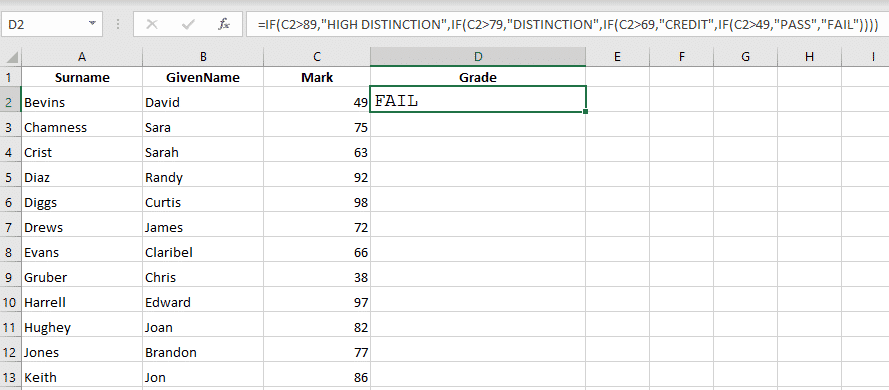
Once we have entered our final condition, including the Value if False, Click OK, and our selected cell should now contain a grade to match the score next to it.
Again, we grab the bottom right-hand corner and drag down to fill the rest of the column with the appropriate grades.
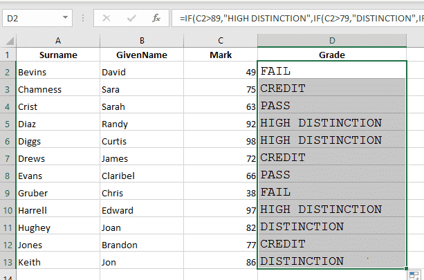
The whole formula is copied down with the relative lookup cell (C2) changing.
IF with other functions
These are just two simple examples of uses of the IF function in Excel. There is a wealth of other things you can do with it, including combining it with other functions, such the SUM, AVERAGE, MIN or MAX functions.
IFS
A recent addition, only in Excel 365 and Excel 2019. It’s an alternative for nested IF statements.
IFS function has matching pairs of conditions and return values. It returns a value that for the first TRUE condition. That means the order of the conditions is important.
=IFS([Something is True1, Value if True1,Something is True2,Value if True2,Something is True3,Value if True3)
Here’s IFS using the same example as above. It’s a lot easier to read and fix.

IF Function alternatives
There are other IF-like functions worth considering.
SWITCH
Another Office 365/2019 function.
It starts with a function then matching pairs of values to test and return value.
SWITCH(Value to switch, Value to match1…[2-126], Value to return if there’s a match1…[2-126], Value to return if there’s no match)
CHOOSE
A long standing Excel function.
It starts with an index value (1 to 254) then a series of values. Choose() returns the nth value from the list.
CHOOSE(index_num, value1, [value2], …)
IFError and IFNA
Two really useful functions for catching errors and problems in cells then returning a nicer message of value than Excel’s # cell errors.
IFERROR() checks a cell for one of these # results; #N/A, #VALUE!, #REF!, #DIV/0!, #NUM!, #NAME?, #NULL!.
=IFERROR (C2, “ Value out of accepted range”)
IFNA() is similar but only catches #N/A errors, not the others accepted by IFERROR().