Excel doesn’t automatically number lists but there are at least six ways to add numbering depending on your needs and how the list appears.
Numbering is important but can be annoying when you’ve got a large dataset. If it’s small, it’s easy to number it manually or by an auto-filling sequence. But if it’s inconsistent (such as blank rows), you might find you need to filter certain parts of the data to stop the numbering can become a complete mess.
Do you need fixed numbering or should the numbering change for a filtered list?
Here are six different ways you can number rows in Excel. For both consistent and inconsistent data, with fixed or changing numbering.
Numbering Rows using Fill Handle
If you have a consistent set of data that doesn’t have any blank rows, you can use the fill handle or even the fill series feature.
Here below, we’ve got a dataset detailing a list of episodes.
To number each row, we can use the Fill Handle.
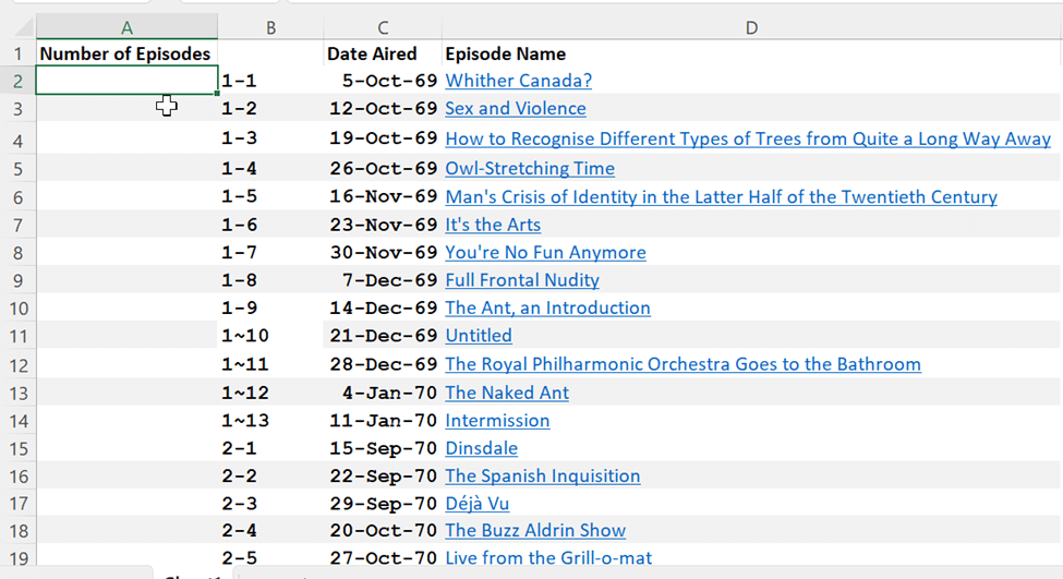
First, you’ll need to fill data in A2 and A3 so that the fill handle can finish the rest.
Place 1 in A2; and 2 in A3.
Highlight cells A2 and A3.
Hover the mouse over the bottom-right corner of A3, a plus icon will appear.

Double-click on the corner, and the remainder of the rows will be filled.

The fill handle will only work if there are no inconsistencies with the data e.g. blank spaces between rows, or if you have a blank column adjacent to where you’re using the fill handle.
Otherwise, you can manually drag the fill handle yourself, but this can become a problem particularly if you’re using a long dataset.
Use Fill Series
Another way to auto-fill data until the end is using the Fill Series feature.
First, you’ll need to find out what the total number of rows there are in the dataset, simply press Ctrl + END to skip to the bottom of the data set, press Ctrl + HOME to return to the top.
Enter 1 into cell A2 then go to Home | Editing | Fill | Series…
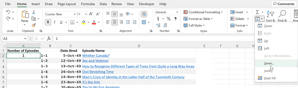
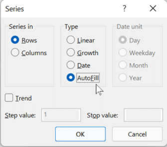
A Series box will pop up.
Under Series in choose Columns
Under Type choose Linear
Ensure Step Value is 1, and Stop Value is set to the total number of rows you found out earlier using Ctrl + END, Remember if you’re using headers, you’ll need to take note of that when inputting the stop value (in our example, 48 rows minus 1).

Then press OK and the data will fill until the last row you’ve stated.

Although it eliminates the need to manually drag, it will include any empty rows, so only really applies for consistent datasets.
Sequence() gives more options
Yet another option is the relatively new Sequence() dynamic array function. Sequence() returns a series of numbers, usually starting with 1. The beauty of Sequence() is the easy access to other options like starting from value, different increments, counting backwards or counting across columns.
All you need to do is give the number of values you need — we’ve used the Row() function to do that.

We’ve filled in all the defaults in the above example:
=SEQUENCE(ROW(A48)-1,1,1,1)
Where cell A48 is the last cell in the list.
All you have to do is enter the first value (the number of rows to fill). All the other parameters are optional and default to one:
=SEQUENCE(ROW(A48)-1)
Sequence() might seem excessive for a simple example and you’d be right. But it’s handy for more complicated situations like:
Starting from another number, for example starting from 26
=SEQUENCE(ROW(A48)-1,1,26,1)
Or incrementing in greater steps e.g. 2:
=SEQUENCE(ROW(A48)-1,1,1,2)
Or even counting backwards, e.g. from 26 backwards, one at a time:
=SEQUENCE(ROW(A27)-1,1,26,-1)
Use COUNTA and IF functions
Another way around it is using a combination of the COUNTA and IF functions in Excel. This option lets you skip blank or other rows you don’t want to number.
For example, with inconsistent data like we can see below, we can add the following in A2
=IF(ISBLANK(B2),"",COUNTA($B$2:B2))
Select your cells then go to Editing | Fill | Series to bring up the Series dialogue box.
Select Type under AutoFill and then press OK.
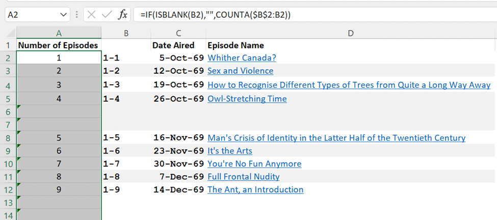
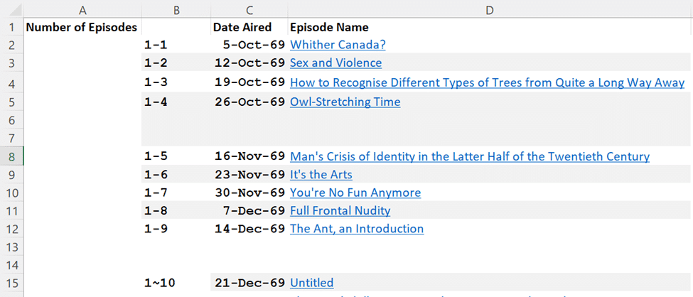
The blank cells will be skipped over, only counting the rows that are filled. It’s also dynamic, so if you end up removing a row, adding etc, the numbering will automatically update. However, if you try filtering the data of any column, it can mess up the data.
Use Subtotal Function
Another way is to use the Subtotal Function in Excel. This is good if you want the numbering to change for filtered lists.
Insert the formula into cell A2
=SUBTOTAL(3,B2:$B$2)

Now you can auto fill handle the remaining cells.
As we can see below, if you decide to filter the data, the row numbering ends up changing automatically in the correct order as well. So if you want to change the row numbering when you filter your data, subtotal function is the way to go.

Row()
Row() returns the row number for the cell you add as a parameter. Row(B3) returns 3 Row(A125) returns 125 and so on.
It’s a simple way to number; all you have to do is subtract the number of rows before the list starts. That’s usually “1” with a list starting in the second row.
=Row(A2)-1 then copy the formula down to the rest of the column.

Easily calculate stock and asset returns in Excel
Three new performance boosts for Excel 365
Clever picture borders in Excel and PowerPoint