Styles in Excel; quick, table, new, modify

You can combine Excel cell formatting into a style, but not like in Word.

Excel has Styles … truly it does. Word has a way to combine formatting attributes of a letter, word or paragraph into a single block with a name like ‘Heading 1’. Excel has a feature also called Styles but it’s a very different animal indeed.

In this article we’ll explain what you can do with Excel styles and why few people, even Microsoft, talks about Excel styles (hint: compared to Word Styles, it’s too embarrassing).

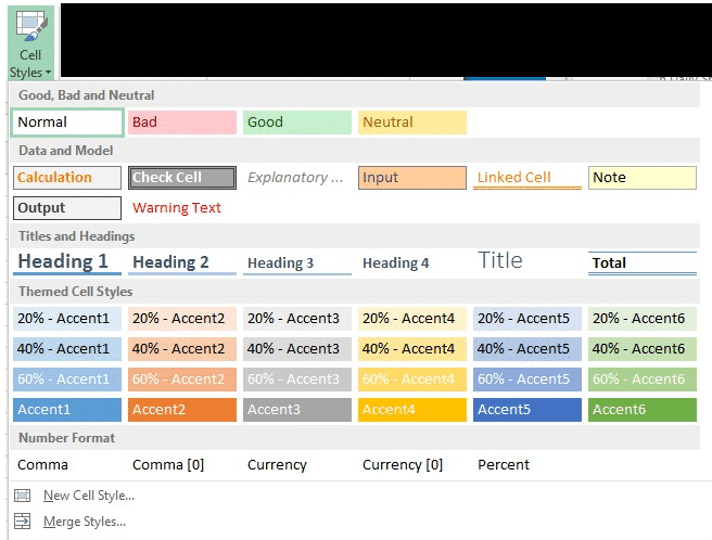
At Home | Style | Cell Styles you can see a range of pre-defined styles.

Quick Style Buttons – Comma, Currency, Percentage

The familiar formatting buttons (Comma, Currency etc.) on the ribbon/toolbar are actually shortcuts to an in-built cell style.

Modify Style

Right-click on a style, say 40% Accent 2 in pink and choose ‘Modify Style’ to see what it does.

As you can see, this style only applies Font and Fill attributes to the cell. Other possibilities like Number, Alignment, Border and Protection aren’t touched by this style. The style name can’t be changed because it’s an in-built style, but styles you make can be named or renamed.

Choose another style like Currency and you can see that it only affects the number formatting.

Let’s see how these two styles ‘40% Accent 2’ Pink and ‘Currency’ work together. Here’s three cells, one has no formatting, the next two have the individual styles while the last cell has ‘40% Accent 2’ applied then ‘Currency’.

The result is what you’d expect, especially in the final combined style cell.

Changing the Currency style (to Danish kronor and 4 decimal places) changes the look of both cells with Currency style, as you’d expect:

But changing the ‘40% Accent 2’ style to another color doesn’t change the bottom cell at all.

Why not? The bottom cell has the ‘40% Accent 2’ style just like the cell above it, so why does it still have the old color.

Excel can only apply a single style to a cell, even if the styles affect different attributes of the cell. When the ‘Currency’ style was applied, Excel copied the existing fill formatting into fixed (non-style) formatting then applied the new style. The link to ‘40% Accent 2’ was broken.

Excel styles are not linked or inherited as in Word. You can’t have a ‘base’ style then apply another style over it, even if the two styles complement each other.

The only way you can apply all the formatting to the bottom right cell is to make a new style.

New Excel Style

Making a new style is easy. In fact it’s more straight-forward than in Word because you don’t have to worry about inheritance from another style. What you create in an Excel style is what you get.

To make a new style, start with an example cell that has, or is close to, the formatting you want:

1. Format a cell the way you want it to look including content formatting, color, border etc.
2. Go to Home | Style | Cell Styles | New Style
3. A style dialog will open with all the cell formatting copied into it.

   

4. As you can see, all the formatting from the selected cell has been copied into the new style.
5. Change the name to something more useful.
6. UNcheck any formatting type you don’t want the style to apply. For example, you might de-select ‘Border’ and ‘Protection’ since they are often applied more broadly.
7. Click on Format … to change any formatting.
8. Click OK to create the style.

Change the style

To change the style settings go to the style gallery at Home | Style | Cell Styles, right-click on the style to see other options, including Modify ….

As you can see, there’s also options to Duplicate an existing style or Delete one entirely,

In addition to cell styles, there are also styles available for tables and PivotTables.

Table Styles

At Home | Styles | Format as Table there’s a gallery of formatting styles.

At the bottom is ‘New Table Style …’ however, unlike cell styles, it doesn’t copy a selected tables attributes into the new style.

You have to setup formatting for all the table elements you need, which can be tiresome.

Possibly a better option is to find a table style that’s nearest to your needs, duplicate the style then make changes to suit you. Find a base style in the Home | Styles | Format as Table | Gallery, right-click and choose Duplicate.

Also on the right-click menu are some other useful options:

• Apply and Clear Formatting – will remove all formatting from the selected table then apply the table style
• Apply and Maintain formatting – will keep the existing formatting and apply the table style ‘over’ it.
• Set As Default – changes the default table style

Using parts of a table style

Table Styles are really a collection of styles for different parts of a table. There’s a style for a header row, bottom/total row, first/left column, general columns and the last/right column. Banded / alternate color rows have their own styles.

Unlike traditional styles you can choose what parts of a Table Style to apply. Click in the table then go to Table Tools | Design | Table Style Options. There you can choose which table style elements should be applied.

Pivot Table Styles

There are also PivotTable styles that work similar to Table Styles.

See Also

• Big numbers rounded in Excel
• Excel 2013 Flash Fill
• Benford’s Law and Excel
• Sparklines in Excel 2010
• Finding Spreadsheet Errors
• Beyond the simple =SUM function in Excel
• Hidden tricks in Excel 2003 – Part 1
• Protecting your Excel worksheet – Part 1