Excel’s PowerQuery has many clever tricks, one of them is merging and matching data from multiple tables into a single table. Combine, clean, and transform data from multiple sources into the single format you need; a table, PivotTable or PivotChart
It’s a simple relational database with relations set to match up the rows in each table.

Excel with PowerQuery (aka Get and Transform) is in Excel 365, Excel 2021, Excel 2019 and Excel 2016.
Join three tables
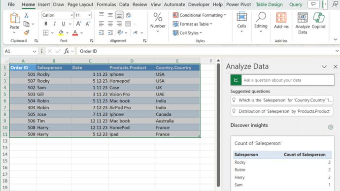
Let’s see how to join three tables based on the common columns “Order ID” and “Salesperson.” Into a single table shown above.
These tables have different numbers of rows. Table 1 has duplicate entries in the “Salesperson” column, while Table 3 contains only unique entries.

It’s advisable to assign descriptive names to each table. This will make it easier to recognize and manage them later. For example, we have named them as Table 1- Orders, Table 2- Products and Table 3- Country.
The column titles don’t have to match across the tables but it makes the connections at lot easier and automatic.
Make Power Query Connections
To create a connection in Power Query, follow these steps:
Select Table 1 (Orders) or any cell in that table. Navigate to Data and click From Table Range under the Get & Transform group

A Power Query Editor pops up, click on the drop-down arrow of the Close & Load button and click the Close and Load To option.
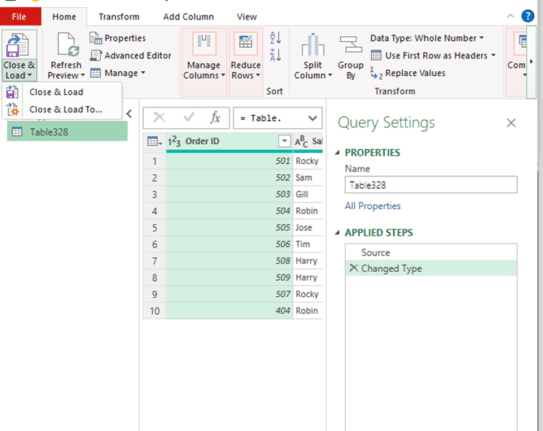
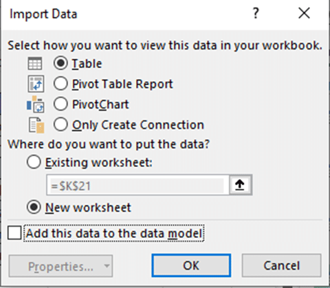
From the Import Data dialog box, select the Only Create Connection option and click OK.
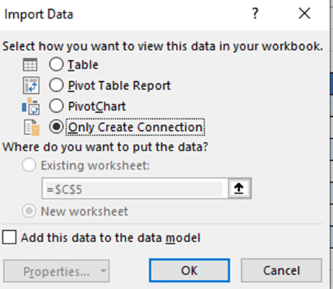
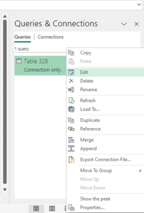
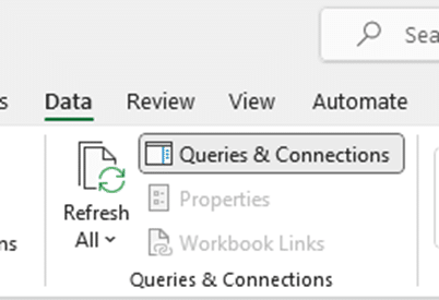
You will notice a connection named after your table/range and this connection will be displayed in the Queries & Connections pane, which appears on the right-hand side of your workbook.

Right-click on the table name and rename it according to your preference.

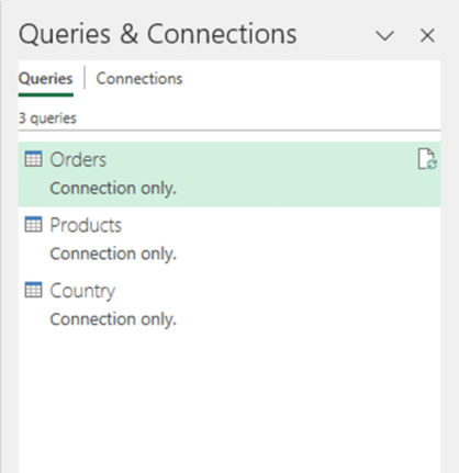
Continue repeating the above steps for all the other two tables you wish to merge (in this case, two more tables: Products and Country). Once completed, you will see all the connections listed in the pane:
Merging Connections into one table
Navigate to the Data tab, within the Get & Transform Data group, click Get Data | Combine Queries | Merge
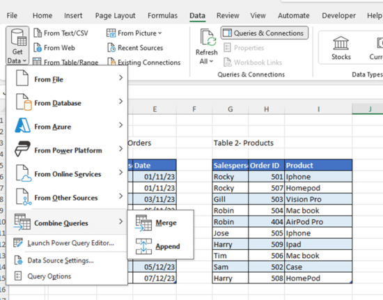
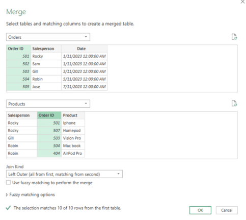
In the Merge dialog box, choose your first table (Orders) from the first drop-down menu and your second table (Products) from the second drop-down menu. In each preview, click on the matching column (Order ID) to select it. The selected column will be highlighted in green.
This where having matching column titles saves a lot of confusion!
In the Join Kind drop-down list, keep the default selection and Click OK.
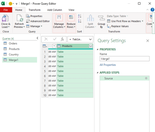
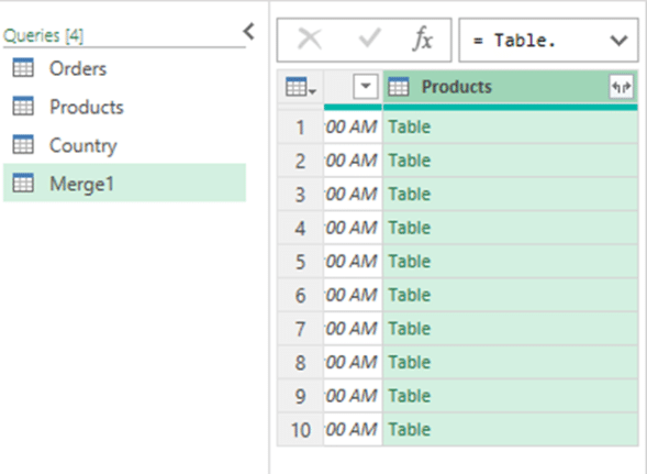
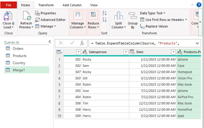
You will notice the Power Query Editor displays your first table (Orders) with an additional column at the end, named after your second table (Products). Initially, this new column will contain the word “Table” in all its cells instead of actual values. Don’t worry, you have done everything correctly.
In the newly added column (Products), click on the two-sided arrow in the header and expand the Product option.
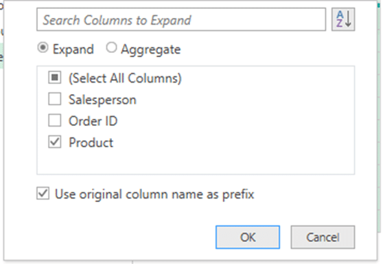
As a result, you will get a new table (Merge 1) that includes every record from your first table along with the additional column(s) from the second table.
Merge more Tables
Now let’s merge Table 3 (Country) with the newly merged Table (Merge 1).
Navigate to Data|Get Data | Combine Queries| Merge
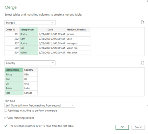
In the Merge dialog box, select your newly merged table (Merge 1) from the first drop-down menu and your third table (Country) from the second drop-down menu. In each preview, click on the matching column (Salesperson) to select it. The selected column will be highlighted in green. In the Join Kind drop-down list, keep the default selection and Click OK.
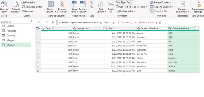
Now you have a merged table that includes the original table along with the additional columns copied from the other two tables. Click the two-sided arrow in the header and expand the column by selecting the Country check box.
Import Merged table to Excel
You can now load the merged PowerQuery table back into Excel. In the Power Query Editor, go to the Home tab, click the Close & Load drop-down arrow, and select Close and Load To. In the Import Data dialog box, select Table and New Worksheet options, then click OK.
Your newly created table with the merged tables is imported into a new worksheet. You are free to adjust the cell formats and customize the default table style to match your preferences.
Update/Refresh the Merged Table
Power Query only requires a one-time setup. When you make changes to any source table, you don’t need to repeat the entire process. Just click the Refresh button on the Queries & Connections pane, and the merged table gets updated instantly.

If the pane has disappeared from your Excel, click the Queries & Connections button on the Data tab to bring it back.
Alternatively, you can click the Refresh button on the Query tab (this tab activates once you select any cell within the merged table).
What to do with the merged table
Now you have a merged table, there’s no end to what you can do. Make PivotTables, PivotCharts or plain old Charts. Home | Analyze Data is a good place to start for a quick look at the highlights.
Download the example file
Subscribers to Office Watch or Office for Mere Mortals can download a complete Excel file with a working example of merged tables.
This download is available EXCLUSIVELY to Office Watch subscribers. The link to this and other special downloads is in each issue of Office Watch or Office for Mere Mortals