Some Excel functions won’t spill their results in the way you might expect. Edate(), EOmonth(), IsEven(), IsOdd() and RandBetween(), among many, need an extra little trick to become a dynamic array function.
We’ve already explained how many common Excel functions (Round(), Trim(), Upper() and many more) can “spill” their results into multiple cells. But then—bam!—you try using a function like Edate() or IsEven()and instead of a neat array of results, Excel hits you with the dreaded #VALUE! error.
So, what’s going on?
Legacy Functions and Their Spill Aversion
The issue boils down to the history of Excel itself. The functions that don’t support spilling—such as , EOmonth(), Weeknum() are from the old “Analysis Toolpak” add-on. These functions have now been included in Excel but weren’t updated to spill in the same way as the core Excel functions. So when you give one of the functions a range like =IsOdd(A2:A6) there’s a #VALUE error.

The problem also appears in newer functions that originated in the Analysis Toolpak like NetWorkDays() and the modern NetWorkDays.Intl() function.
The fix is incredibly simple – add a + plus sign to the start of the range. Instead of =IsOdd(A2:A6) use =IsOdd(+A2:A6) .
Why It Works
The + operator triggers Excel to convert the range into a numeric array. Once coerced into an array, the function is suddenly happy to process it element by element, returning a spilled array of results just like newer dynamic array functions do.
EOMONTH
Basically this function returns the last day of the month, a specified number of months before or after a given date. Excel can evaluate these functions across a range—it just needs a little nudge. That nudge comes in the form of a + sign.
Try this:
=EOMONTH(+A2:A6, 1)
That small plus sign is more than it looks—it tells Excel to treat the range as an array. It forces Excel to evaluate the reference in array context, which triggers spilling behaviour even for functions that don’t natively support dynamic arrays.

Other Functions You Can Fix This Way
This trick doesn’t just work with only EOMONTH. You can apply it to many legacy functions that were never designed with dynamic arrays in mind, such as WEEKNUM, EDATE, WORKDAY, NETWORKDAYS.
WEEKNUM
This function returns the week number for a given date—based on how the year is divided into weeks.
Suppose you want to get the week number of each date in A2:A6.
=WEEKNUM(+A2:A6)

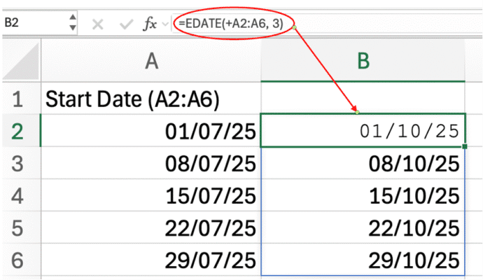
EDATE
This function returns the date that’s 3 months ahead of each date in A2:A6.
=EDATE(+A2:A6, 3)
WORKDAY
Suppose you want to calculate the workday, 10 days after each start date in A2:A6, excluding weekends.
=WORKDAY(+A2:A6, 10)

NETWORKDAYS
Suppose you want to count the number of working days between each date in A2:A6 and today.
=NETWORKDAYS(A2:A6, TODAY())

You can also use this technique inside newer dynamic array functions for even more flexibility, like:
=TEXT(EOMONTH(+A2:A6, 1), "mmm yyyy")
This will spill a list of month names based on the end of next month for each date.
Excel’s dynamic arrays have revolutionized how we build formulas—but older functions still carry some baggage. Fortunately, a simple plus sign is often all it takes to bridge the gap between old and new.