Display scores or ratings visually in Excel using solid and hollow emojis or symbols, you can use a combination of simple formulas and conditional formatting. This approach is useful for representing ratings, progress, or performance in an intuitive and engaging way.
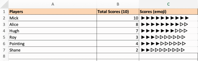
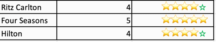
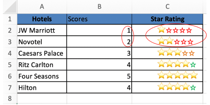
With a little Excel trickery, you can show multi-colored symbols with alternates for the ‘missing’ scores like this:
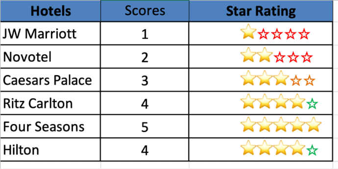
The ‘empty’ icons can even change color depending on the value. The red hollow stars for ratings 1-3 but green for the higher rated rows.
Simple star symbols
Let’s start with simply converting a rating or value into symbols or emoji.
Excel supports Unicode characters, including solid (⭐) and hollow (☆) emojis. You can manually input them or use REPT formulas to generate them dynamically.
The REPT() function in Excel repeats a specified character or text based on the numeric values.
The syntax for REPT is:
REPT(text, number_times) where Text represents the character or string to repeat.
number_times represents the number of times to repeat the character.
For Example: =REPT("⭐", 5).
This formula fills solid stars ⭐⭐⭐⭐⭐ (5 solid stars).
Note: To display a score visually, you can use Unicode Characters:
Solid star (⭐) – Unicode U+2B50
Hollow star (☆) – Unicode U+2606
Windows: Press Windows + R, type charmap, and hit Enter or Win + . (period/fullstop) for the Emoji Panel.
Mac users : Press Control + Command + Space to open the Character Viewer.
Search for ” Unicode U+B250″ or “⭐” in the search bar and click insert to use the emoji.
Using Solid and Hollow Emoji for Scores
Now let’s expand on that to show different symbols for the actual rating and the rest up to the top value.
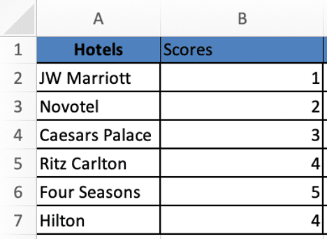
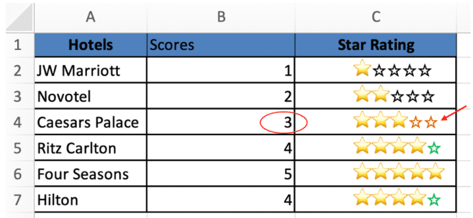
To start with launch Microsoft Excel, In Column A, enter Hotels name and Column B, enter scores.
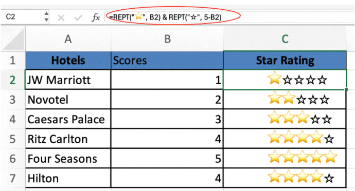
NextClick on Cell C2 (or any cell next to the first score) and enter the formula:
=REPT ("⭐", B2) & REPT("☆", 5-B2) Press Enter. Click and drag the fill handle down to apply the formula to the other rows.
=REPT("☆", 5-B2) – ‘5’ is the top value in the scale subtract the actual value to get the number of ‘missing’ or ‘not received’ symbols.
Extending to a 10-Point Scale
For a score out of 10, lets adjust the formula a bit. Change the ‘5’ to ‘10’.
=REPT("►", B2) & REPT("▷", 10-B2)
If B3 = 8, the output will be ►►►►►►►►▷▷ (8 solid, 2 hollow).
REPT("►", B2): Repeats the solid emoji B2 times (B2 contains the score).
REPT("▷", 10-B3): Fills the remaining spots with hollow emoji.
Do that with any combination of symbols you like.
Apply Custom Formatting
Select the cells containing the emojis (e.g., C2:C7). In the formula bar, highlight the solid stars by clicking and dragging over them. Go to the Home tab, then click Font Colour, and choose a colour you like. Optionally, you can make the stars bold and increase the font size (e.g., 12pt) for better visibility.
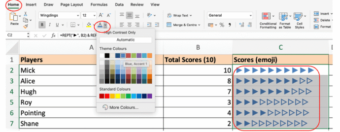
To ensure the emojis align properly, change the font to Calibri, Consolas, Courier New, or any other monospaced or emoji-friendly font of your choice.
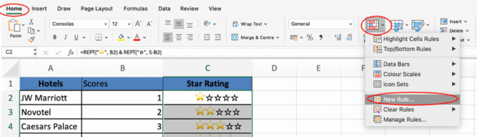
Apply conditional formatting using solid and hollow emojis
To get even fancier, use conditional formatting to change the color of some symbols.
Although colors and icons are frequently used for visual cues, one of the most creative and intuitive ways to represent data is with solid and hollow emojis—especially stars like ⭐ (solid) and ☆ (hollow).
let’s explore how to use conditional formatting to color-code results based on data ranges.
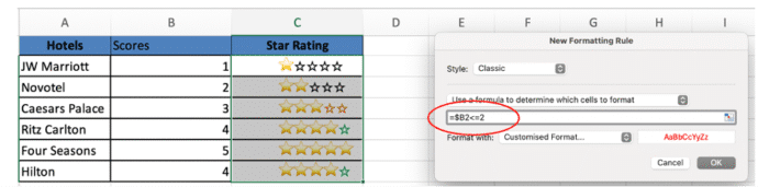
Select the Stars column (e.g., C2:C7).Go toHome | Conditional Formatting | New Rule
In the New Formatting Rule window, set the Style to Classic, then choose “Use a formula to determine which cells to format” from the dropdown below.
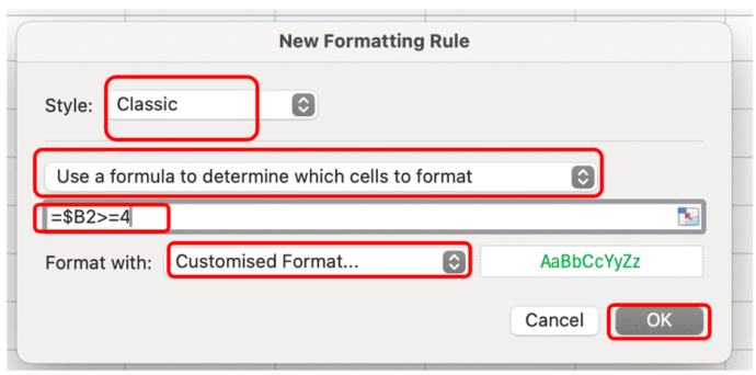
Use the Format with dropdown to choose any color you like. You can also apply bold styling if you prefer.
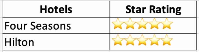
Suppose you want to colour the hollow star in green for high scores (4–5), enter the formula:=$B2>=4 This will format the hollow stars in green.
That works because the yellow ‘solid’ stars are image emoji with a fixed color but the ‘hollow’ stars are text that Excel can change the color. Conditional formatting is changing the color of the whole cell but only the ‘hollow’ text is affected.
For using Yellow colour for hollow emoji for medium score (3); enter the formula=$B2=3.
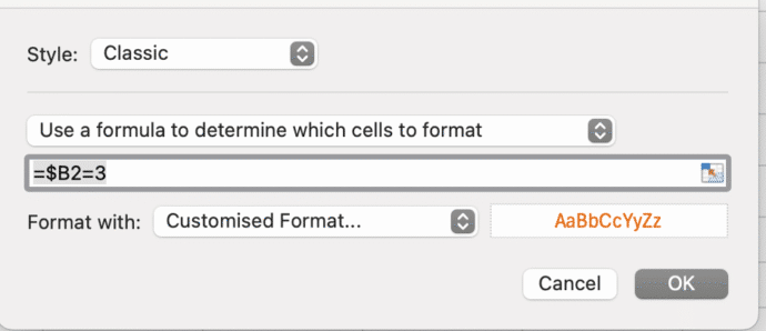
This will format the stars in orange.
For Red stars for low score (1-2); enter the formula =$B2<=2
This will format the Stars in red.
This is how by leveraging simple formulas, conditional formatting, or Unicode characters, you can create a dynamic and visually appealing score representation.