Microsoft Excel, Microsoft Office, Microsoft Office for Mac, Office 2007, Office 2010, Office 2013, Office 2016, Office 2019, Office 365 /

Stop accidental duplicates in your Excel lists or Tables

7 September 2020

Stop duplicate names, email addresses or product SKU’s from being added to an Excel list or Table. Adding more rows to an Excel Tables can be done while preventing accidental duplicates creeping into the list.

Excel Tables or lists can grow to hundreds or thousands of rows, there’s a risk of someone entering a duplicate entry without bothering to check if the person, event or product is already in the list.

We’ll look at ways to stop duplicates being entered with a spot of real-time data entry validation.

Stop Duplicates in a single column

Let’s start with a simple example with a list of first names.

To make sure there isn’t another person with the first name added to the list follow these steps.

Select the data cells. Start with the first data cell in the column (A2 in this case) and extend the selection to the end of the table or the entire column if not using a table. Selecting from the first cell is important.
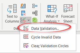
Go to Data | Data Tools | Data Validation.

Allow: select ‘Custom’ then Ignore blank.
Enter the formula =COUNTIF($A:$A,A2)=1 . Change the A references to the column you’re using. We’ll explain that code in a moment.

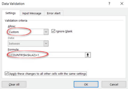
Select ‘Apply these changes to all other cells with the same settings’.
Click OK to apply the data validation.

Now when we enter the next name/row we’ll get an error message for any duplicate. Anyone up on their moon landing history knows there were two Alan’s to step onto the lunar surface in a row (Alan Bean, LMP on Apollo 12 then Alan Shepard, Commander on Apollo 14).