Excel Charts can be even better looking by completely replacing those plain color blocks with pictures.
We’ve already shown how to overlay an Excel Chart with an image now we’ll replace the block with a picture.

Although commonly differentiated by differing colors like this, how about we look at different images instead?
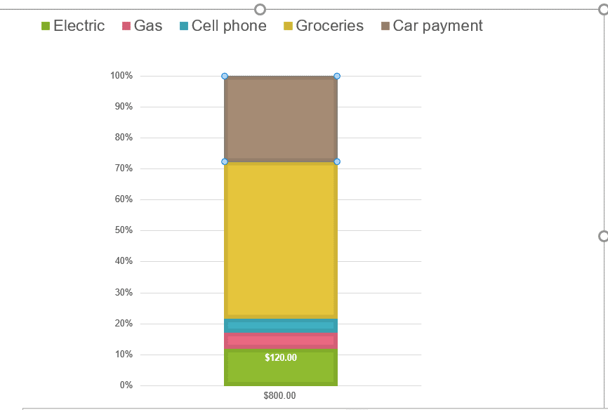
First, click on the plot area within the column, here we’ve selected the brown ‘Car Payment’. This will display the adding the Chart Design and Format tabs to the top ribbon.
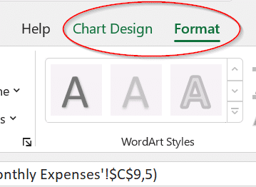
Go to Format | Shape Fill | Picture
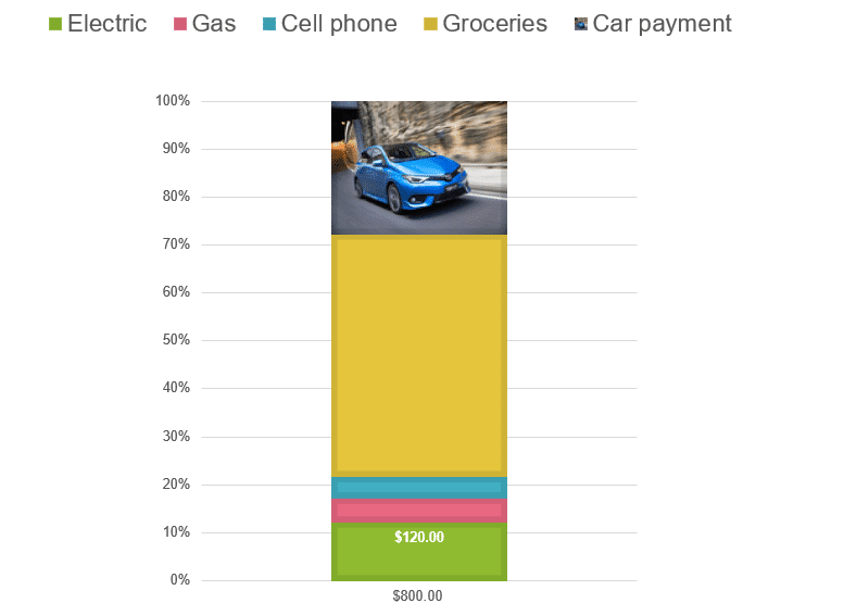
From here it will give you the choice to choose between a file on your computer, stock images, online pictures or icons. Choose your preferred image and double click on it to insert into your graph like so. Make sure you’re choosing the right image that will still reflect the right information in your chart. The examples below still allows users to see the right information but more easily see what’s the car share of the total.
Fixing image proportions
If the image is too stretched out within the area within your graph as shown below, Excel has different ways to format the filled area within the data point.

Go to Format | Format Selection | Fill & Line
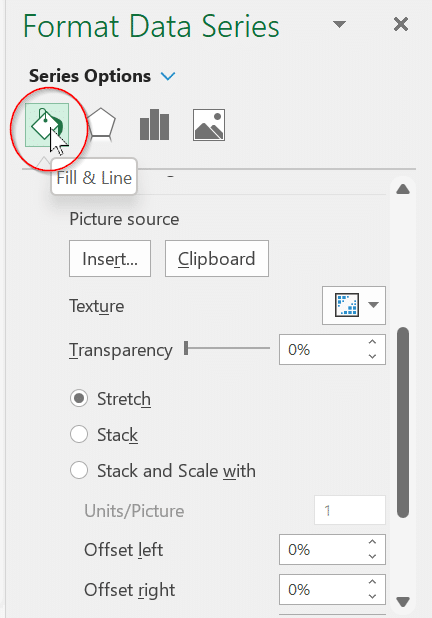
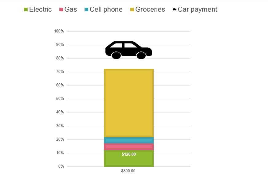
Now you can adjust the transparency, and choose between Stretch, Stack or Stack and Scale with.
Stretch is usually the default option, but if you choose Stack or Stack and Scale with, this will give the option to copy the image multiple times within the filled area, within giving that ‘stretched look’.
Within the same section, users can also add a border around their images and customise their borders choosing between solid, gradient lines, dash type, transparency, color and width.

The images will even update within the Legends above the chart.

Removing a picture from a chart
You may want to remove a picture from a chart, luckily, it’s a no-brainer.
If a picture was simply inserted into a chart, just select the picture with your mouse and hit delete.
However, users must beware, if the picture was filled within a chart element and you follow this method, it will completely delete the data point area.
Instead, users need to select the chart element area and go to Format | Current Selection | Reset to Match Style.
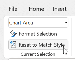
This will return the selection to its original fill effects.
Otherwise, you can also go to Format | Fill & Line | Fill | Automatic.
Make better Office SmartArt by adding pictures