Aggregate() is the grown up version ‘all in one’ function that can replace common functions like Sum() and Subtotal() plus powerful options not available in those older functions.
AGGREGATE() function is a more advanced alternative to the SUBTOTAL function, offering significantly expanded capabilities. Almost an ‘all in one’ solution instead of using multiple functions.
- Aggregate() supports 19 different operations, ranging from basic calculations like SUM and AVERAGE to more advanced ones such as PRODUCT and STANDARD DEVIATION.
- LARGE and SMALL operations can show not just the most extreme values, but also the near-extreme like the second-largest or third-smallest.
- 8 options for managing errors and hidden data, enabling smooth calculations even when error values are present.
- Aggregate() can skip over hidden rows, which makes it especially effective for filtered or dynamic data.
- AGGREGATE can also handle nested AGGREGATE or SUBTOTAL functions, unlike Subtotal()
It’s available in all recent Excel’s including Excel on the web (since at least Excel 2016 for Windows and Excel 2021 for Mac).
The AGGREGATE function comes in two forms:
the reference form =AGGREGATE(function_num, options, ref1, [ref2], …)
and the array form =AGGREGATE(function_num, options, array, [k])
Calculation type by number
Start Aggregate() by telling it which type of calculation to make. Each function / calculation has a number but you don’t have to memorise them because a drop-down list appears in the formula bar.
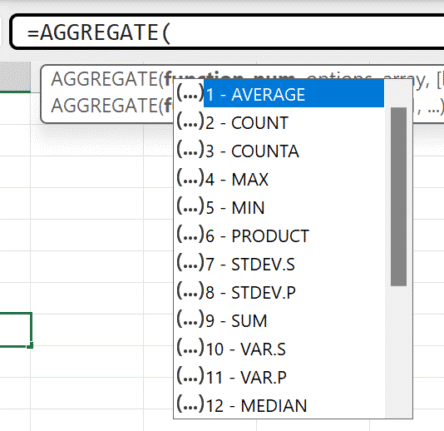
Available Aggregate calculations:
1 = AVERAGE
2 = COUNT
4 = MAX
5 = MIN
6 = PRODUCT
7 = STDEV.S
8 = STDEV.P
9 = SUM
10 = VAR.S
11 = VAR.P
12 = MEDIAN
13 = MODE.SNGL
14 = LARGE
15 = SMALL
16 = PERCENTILE.INC
17 = QUARTILE.INC
18 = PERCENTILE.EXC
19 = QUARTILE.EXC
Options
The options argument Controls how errors and hidden rows are handled during the calculation. This is incredibly useful in tables with filters, errors and subtotals.
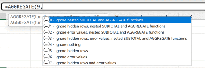
0 – Ignore nested SUBTOTAL and AGGREGATE functions
1 – Ignore hidden rows, nested SUBTOTAL and AGGREGATE functions
2 – Ignore error values, nested SUBTOTAL and AGGREGATE functions
3 – Ignore hidden rows, error values, nested SUBTOTAL and AGGREGATE functions
4 – Ignore nothing
5 – Ignore hidden rows
6 – Ignore error values
7 – Ignore hidden rows and error values
Other Parameters
Then, tell Aggegrate what cells, range or array to get values from.
Ref1 (required): The primary range of data to which the function will be applied.
Array (required): The set of values or an array formula used in the function.
Ref2 (optional): Additional ranges of cells. You can include up to 252 additional ranges.
And finally
The last parameter is needed with some functions.
[k] (optional): Used with functions like LARGE, SMALL, PERCENTILE, and others that need a ranking or percentile value.
With LARGE (14), the [k] chooses which to select – 1 = Largest 2 = second largest 3 = third largest
With SMALL (15), the [k] chooses which to select – 1 = Smallest 2 = second smallest 3 = third smallest
You don’t need to worry about choosing the correct format—in the formula bar, Excel automatically selects the right one based on the function number (function_num) you specify.
Let’s check out few examples on the usage of AGGREGATE function in Excel.
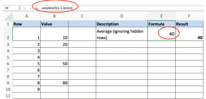
Ignore Hidden Rows When Calculating AVERAGE
When using aggregate functions like AVERAGE in Excel, hidden rows are usually included by default in the calculation. However, sometimes you want to ignore hidden rows (i.e., rows hidden manually or by filters). Below is the formula for doing so:
=AGGREGATE(1, 5, B2:B10)1 signifies AVERAGE,
5 signifies Ignore hidden rows and
B2:B10 = the range of data.
This will calculate the average of the visible cells in the range, ignoring any rows that are hidden manually (not filtered)
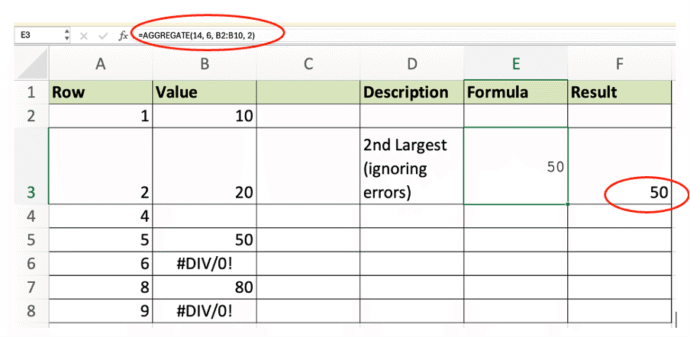
Find the 2nd Largest Value While Ignoring Errors
You can fetch the 2nd largest numeric value from a list, while ignoring any error values (like #DIV/0!, #N/A, etc.).
Formula:
=AGGREGATE(14, 6, B2:B10, 2)1 signifies LARGE, 6 = Ignore error values, B2:B10 = Range of data, 2 =Return the 2nd largest value useful when your data might include #DIV/0!, #N/A, or other errors, but you still want to find the 2nd highest value among the valid entries.
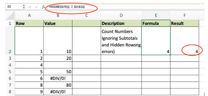
Count Numbers Ignoring Subtotals and Hidden Rows
You can count numbers in a range while ignoring subtotals and hidden rows in Excel, by using the AGGREGATE function
=AGGREGATE(2, 7, B2:B10)2 signifies COUNT, 7 = Ignore hidden rows and nested SUBTOTAL or AGGREGATE results
This ensures your count only includes visible and valid data, skipping over subtotal rows.
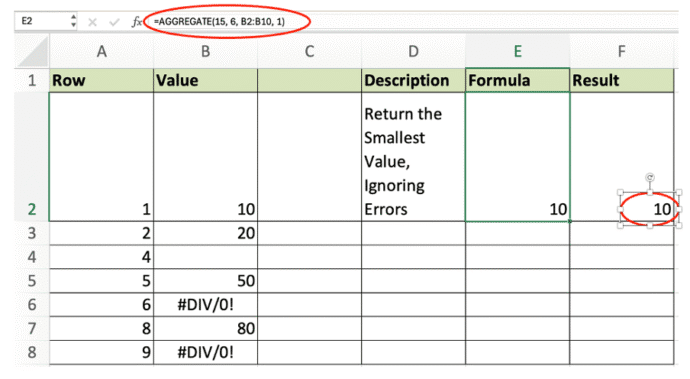
Return the Smallest Value, Ignoring Errors
You can find the smallest numeric value in a range, but ignore any error values like #DIV/0!, #N/A, etc. Simply use the formula:
=AGGREGATE(15, 6, B2:B10, 1)- = SMALL, 6 = Ignore errors, B2:B10 = Data range, 1 = Return the smallest (1st smallest) value.
This is ideal when you’re working with datasets where some values may be invalid due to calculation issues.