There are two a simple ways to make a list of unique or non-duplicate entries from a longer list. Unlike the many automatic ‘unique’ options in Excel, these options work only once but it’s available in many Excel releases, old and new.
Advanced Filter
One is hiding at Data | Sort & Filter | Advanced

Click on Advanced to see the Advanced Filter dialog. It has an option to filter the selected list directly. More commonly ‘Copy to another location’ keeps the original list untouched and makes a copy with only selected items.

List Range: the source list. Like many Excel dialogs, it’s faster to select the range before opening the dialog.
Criteria Range: a filter to apply, if any.
Copy to: where to put the results, after filtering.
Unique Records only
That little check box at the bottom is all you need to copy a list of unique no-duplicates record.

Copies this list of dwarves.

You could add a filter criteria as well. For example criteria to show names with sales above a certain value AND unique records.
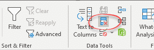
Remove Duplicates
The other de-duplication option is nearby at Data | Data Tools | Remove Duplicates.
Remove Duplicates works by trimming the selected list, so make a copy of the table or cells first.
Select the table/cells then Data| Remove Duplicates. Choose the column with the duplicates.

The result is a shorter list with no duplicates.

If you’re sure that a ‘one-off’ copy is enough, use Advanced Filter or Remove Duplicates. Overall it’s better and safer to use a method which is automatically updated when the source list changes.
Unique() makes a once difficult task really easy in Excel
Extend UNIQUE() for distinct values that appear more than once