Microsoft 365, Microsoft Excel, Microsoft Office, Microsoft Office for Mac, Office 2007, Office 2010, Office 2013, Office 2016, Office 2019, Office 2021 / Office LTSC, Office 365 /

Six clever tricks (at least) in Excel's Name Box

by Megan Casey 13 January 2023

I found at least six uses for the Excel Name Box beyond just displaying the current cell address. The Name Box is an unassuming little box at the top of your Excel worksheet that you may not have thought about much, but it has a powerful range of uses for selecting and moving around a workbook.

The Name Box can do a whole lot more than just display the current cell reference. Microsoft developers have packed a lot of nifty tricks into the Name Box and I’m going to explore some of its uses in this article.

Make or view a selection

Name Box doesn’t just display the current selection or named range, it lets you select a range or selection. There are some tricks to make cell selections by typing instead of dragging a mouse around.

Display the Address of a Cell or Cells

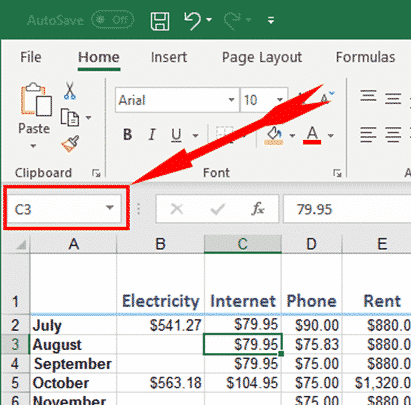
The simplest thing the Name Box does is display the address of the cell you have selected. But what if you select more than one cell?

If you select a range of cells, the Name Box will display the address of the first cell in the range. Note, however, that the ‘first’ cell in the range depends on where you first clicked and which direction you dragged to make the selection. So if I have selected the cells from C4 to F10, the address in the name box will depend on which cell I started to drag from.

Dragging from C4 to F10:

Dragging from F10 to C4:

If you select a number of non-contiguous cells (using Control-click), the Name Box will display the address of the last cell you clicked on.

Display the Number of Rows and Cells Selected

If you think it’s of limited use to see where you started selecting a range of cells, back up one step, as the Name Box shows you something quite interesting before you release the mouse button. If you select a range of cells, and keep the mouse button held down, you will see the number of rows (R) and columns (C) that you have selected. So in the range we selected above, C4 to F10, we have six rows and four columns.

Use the Name Box to Select Cells

While seeing which cells you have selected is interesting, a much more useful function of the Name Box is to go in the other direction – to use the box as a quick way to select cells.

At the most basic level, just type a cell address in the Name Box and hit Enter, and the cursor will jump to that cell.

To select a range of cells, type the two cell addresses separated by a colon.

For example, to select all of the numerical data cells in our sample file, we would double-click in the Name Box (to highlight whatever is already in there), type B2:F13 and hit Enter, after which our worksheet would look like this:

To select a number of non-contiguous cells, we type each of the cell addresses in, separated by commas. So in our sample file, if we want to select only the cells that have a figure in them for electricity, we would type B2,B5,B8,B11 and press Enter.

By combining colons and commas, we can also select multiple ranges of cells.

Colons: separate start and end of a range

Comma, separate ranges

Select all the figures for the first and last quarter in our worksheet, we would type B2:F4,B11:F13.

We can even use the Name Box to select cells on a different worksheet and take us to that worksheet. To do that type the worksheet name followed by an exclamation mark (!), then the cells we want to select.

So if we have a similar table of figures on Worksheet 3, and we want to select all the figures from the first quarter on that worksheet, we would type Sheet3!B2:F4.

Select Rows or Columns

As well as selecting individual cells and ranges of cells, you can also use the Name Box to select particular rows or columns.

To select all of the row you’re currently in, type R then Enter.

To select all of the column you’re currently in, type C then Enter.

To select a range of rows, type the first and last row number separated by a colon.

For example 2:4 would look like this, selecting all of rows 2,3 and 4 only.

To select a range of columns, type the first and last column letter, separated by a colon.

For example, B:F would look like this, selecting all of columns B through F.

NOTE: You must enter at least two rows or columns here. If you enter just a single letter or number, and error will be displayed.

You can also select both rows and columns at the same time.

To select all of a range of rows and columns, enter the two ranges, separated by a comma.

So if I enter 2:4,B:F, the whole of rows 2 to 4, and the whole of columns B to F will be selected:

Intersecting Ranges

You can also select only the area where the ranges of rows and columns intersect. To do this, we enter the two ranges again, but this time, we separate them with a space.

So if I enter 2:4 B:F the selection will look like this, selecting only the cells in rows 2,3 or 4 which are also in columns B through F.

Make Room!

The Name Box seems too small but it can be much longer.

Click on the three vertical dots and drag /left/right to change the width of the Name Box.

Look for the cursor as a double-arrow.

Copy and Paste

Anything in the Name Box is just a string of text. It can be copied and pasted, just like Formulas can.

That’s really useful if you’re copying a range from one worksheet to another. Or cloning with some small adjustments.

If necessary, copy a cell reference from the Name Box, paste it somewhere else to edit then paste back into the Name Box. Very useful for longer strings that don’t appear in the small box.

Named Ranges and Objects in the Excel Name Box
Excel convert Range to Array in VBA
LET() assigns names to calculations in Excel
Faster SumIFS in Excel 365 for Windows