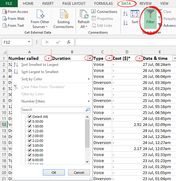
Any Excel worksheet that has lists with headings on the top row can quickly get pull-down menus to filter or sort the data.
For a regular Excel worksheet, go to the Data tab and click the Filter button. This adds extra pull-down menus to each of the headings.

For an Excel Table, the filter buttons appear automatically as the table is created.
Data Filter options
Either way, there’s a lot of power hiding under those little buttons. There are many options to sort and filter the list.
Sort – ascending or descending
Sort by … – leads to the Custom Sort dialog for multi-column sorting rules.
Clear Filter – removes all filters and displays all rows.
Text Filters – make filtering expressions: Equals, Does not Equal, Begins with, Ends with, Contains, Does not Contain, Custom Filter.
Number Filters – Equals, Does not Equal, Greater Than, Greater than or equal to, Less Than, Less Than or Equal to, Between, Top 10, Above Average, Below Average, Custom Filter.
Then there’s a list of all the items in the list, you can check/uncheck the rows to show.
Any filtered column gets a little ‘funnel’ icon on the top row.

Turn off the filter buttons
Excel Tables get the data filters added automatically but sometimes they aren’t needed or just get in the way.
Easily fixed. Click in the table then go to the Table Design tab | Table Style Options and turn off ‘Filter Button’.

Five ways to turn text into Excel dates
Excel Conditional Formatting, beyond the pre-sets
What are Excel Tables and why you should use them
Solved! The problem with Excel Tables and Transpose