Excel has some nifty and simple options for color highlights the extremes in a list of values. It’s called Conditional Formatting and you can do all sorts of clever things with it.
First let’s look at the simple presets that Microsoft has given us, some of the obvious choices they’ve left out and how to make the limited presets work in the real world.
Here’s a simple list of values.

It’s hard to immediately see which is the lowest and highest until you apply some conditional formatting:

Now it’s easier to tell that Alan is the lowest and Walter is the highest value.
That’s done by selecting the column of numbers then Conditional Formatting from the Home tab.

The choices are bewildering but Excel has Live Preview to make selection easier. As you hover over each choice, the selected cells will change to see how that choice will look.

There’s all sorts of options to play with. Data Bars, Color Scales, Icons, Shapes, Ratings and so on. You can check those out for yourself with Live Preview to make it quite painless.
Let’s look at how Microsoft’s presets let their customers down. As with many Office features, the presets are designed to look good in product demonstrations and impress novices.
In daily use there’s some presets and options that even occasional users would like to have. Let’s look at some and how to do it.
Highest and lowest value
The color scales are a great idea but often you don’t want the entire spectrum of color – just highlight the highest and lowest values.
That’s easy to do using the Conditional Formatting | Top/Bottom Rules | Top 10 items … and changing the default ‘Top 10’ to just 1.

With the same group of cells selected, choose Conditional Formatting | Top/Bottom Rules | Bottom 10 items … and change the Bottom value to 1.

Change the formatting to another selection or a Custom Format.
Now the lowest and highest values are highlighted and automatically update when the values change.

Outside the value range
Often you have a situation where values are supposed to be within a certain range. For example older than 18 but younger than 60 years.
There’s two ways to handle this. Use the Highlight Cells Rules for both Greater Than and Less Than to set the range. You can have the same color setting or different colors for higher and lower values.

Or, highlight the values within the accepted range with Highlight Cells Rules | Between:

Using Cell Values
It’s better and more flexible if you don’t ‘hard code’ the values in conditional formatting. Better to link them to cells that you can more easily change. This also makes the conditional formatting more obvious to anyone using the worksheet. (conditional formatting can hide away on a worksheet then pop-up unexpectedly and without explanation).

To use a cell, click in the value box then click the cell you want to link with. Excel will add the cell reference as an absolute reference.
Even better a Range Name instead of a cell reference. That will be clearer to anyone trying to figure out the logic in future.

Apply color to other cells
Microsoft’s concept of conditional formatting is quite limited. It assumes that you want to apply colors only to the cell that holds the value. But that’s not always the case.
It’s quite reasonable to want a whole row or column to be highlighted when a value is reached. In our small example, you might like the name to get the same formatting as the value cell.
That’s possible, but not as easily done as you’d like.
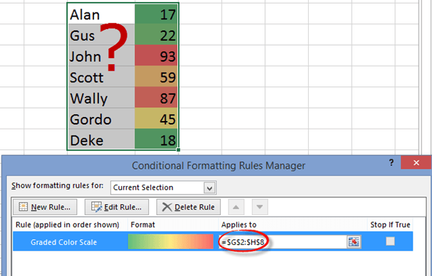
Here we’ve selected the two columns, name and value, then chosen Conditional Formatting | Color Scale. Even though the ‘Applies to’ range is both columns, only the value cells are changed.

Microsoft would probably argue that’s how Excel is supposed to behave but we consider it a bug and a long-standing one.
You can apply conditional formatting to other cells like this:
Select all cells to be formatted then go to Conditional Formatting | New Rule. Select rule type ‘Use a formula to determine which cells to format’.

Enter the formula to check against. As you can see, the column is an absolute reference ‘$H’ and the row isn’t ‘2’ so the row used in the formula will change for each row.
Here’s the result with two Conditional Formatting rules, one each for upper and lower age limit. The formatting is applied to the name/label cell as well as the value cell.

Excel is getting better Conditional Formatting with much needed improvements
Justify, Fill, Orientation, Shrink to Fit and other Excel formatting tricks.
Six choices for removing formatting and more in Excel
Text and formatting tricks for Excel