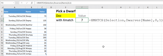
XMatch() function in Excel locates an item in an array or range of cells, then returns its position relative to the item. It’s similar to XLookup() which returns the cell value while XMatch returns a relative position in the array.
Syntax
=XMATCH(lookup_value, lookup_array, [match_mode], [search_mode])
Arguments
- Lookup_value – the value to find.
- Lookup_array – the range/table to search
- [match_mode] – specify the match type.
- 0 – the exact match (default setting)
- -1 – the exact match or next smallest match
- 1 – the exact match or next largest match
- 2 – the wildcard match (*, ?, ~)
- [search_mode] – specify the search type.
- 0 – search first to last (default setting)
- -1 – search last to first (reverse search)
- 2 – Perform a binary search based on the ascending order of the lookup array. Invalid results are returned if not sorted.
- – 2 – Perform a binary search based on the descending order of the lookup array. Invalid results are returned if not sorted.
It’s an improved version of the old Match() which doesn’t have a wildcard option nor search mode parameter.
XMatch – Exact match example
Supposedly you had a list of names, and you wanted to find the position of “Doc” in the list of names within the range C2:C14. The formula for this would be:
=XMATCH(E2,B2:B14,0,1)
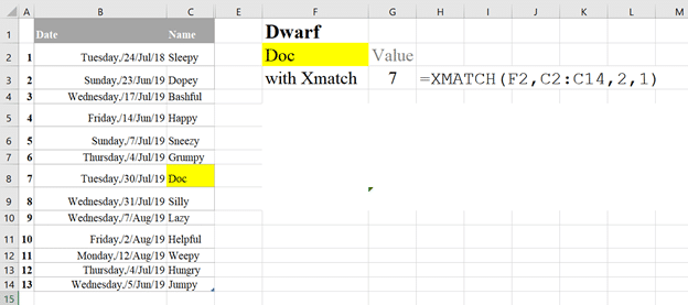
This will return the value 7.
If a name is placed in cell F2 that isn’t within the range C2:C14, Excel will return the value #N/A.
Match_Mode Example – Using Wildcard (2)
When the Match_Mode has been set to 2 within the XMatch formula, this will specify the match type via wildcards.
Excel has three kinds of wildcards that you can use within your formulas. Two are quite standard but the ‘escape’ character is unusual.
- Asterisk (*) which finds any number of characters e.g. s*t will find “sat” and “start”.
- Question mark (?) which finds any single character e.g. s*t will find “sat” and “sit”.
- Tilde (~) followed by ?, * or ~ to find question marks, asterisks or other tilde characters, e.g. st~? will find “st?”
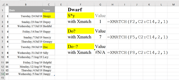
Here, we’ve provided examples of each type which returns different results.
Note: for S*y (F2), Excel will return the first name that begins with S and ends with Y within the range, so it has returned the value of 1 rather than 5 or 8 (It cannot produce multiple values).
For Do~? There are no names within the array that displays ‘?’ so, as there is no result, Excel will return #N/A.
Search_Mode Example – Using Reverse Search (-1)
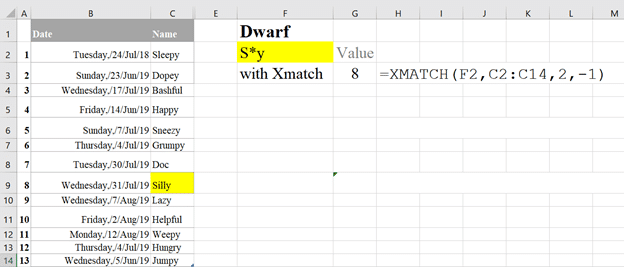
Using this search mode, XMATCH compares the value being looked up against the lookup array, starting with the last value and working towards the first value.
Like using our previous example, if we use Reverse Search in the search mode, Excel will look from the name Jumpy right up to Sleepy.
This means that Excel will return the value of =XMATCH(F2,C2:C14,2,-1) as 8. As it will count the name Silly as the first value to recognize within the list of names as it is working from bottom to top. Note it will still produce the value on the list from top to bottom, so it still understands that the value is in 8th position.
Case Sensitivity
XMatch() is NOT case sensitive, meaning that using Capital or Lower-case letters will not have an effect on the result.
Combining Xmatch() with the Exact() function will ensure that case sensitive matches are performed.
=XMATCH (TRUE,EXACT(lookup_value, lookup_array, [match_mode])
If the letters do not match exactly, Excel will return #N/A instead of a value.
Differences between XMATCH and MATCH?
Xmatch() has a lot more adaptability and capability than Match(). It can replace Match () in some situations. The syntax in exact matches is very similar, for instance:
=XMATCH(lookup_value, lookup_array, [match_mode], [search_mode])
=MATCH(lookup_value, lookup_array, [match_type])
As shown in the example below, it will produce the same results based on using the default for Xmatch() search mode (1).
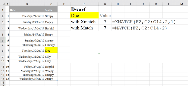
Match() does not offer the search mode argument that controls the match behaviour.
Match_type offers different numbers indicating which value to return. Such as 1, which indicates the exact match or next smallest match (the values must be in ascending order).
However number 1 in Match_mode will search the exact match or next largest match. Additionally, the list of values do not have to be ascending in order to calculate correctly – an added bonus.
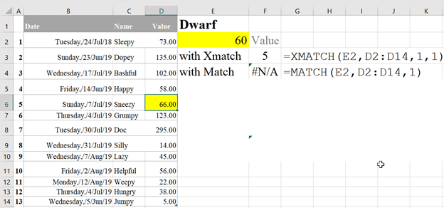
For example, if we use both formulas within the list of values below, XMATCH will return the value 5 (which is the next largest match to 60 on the list), MATCH will return the value #N/A as the data isn’t ascending.
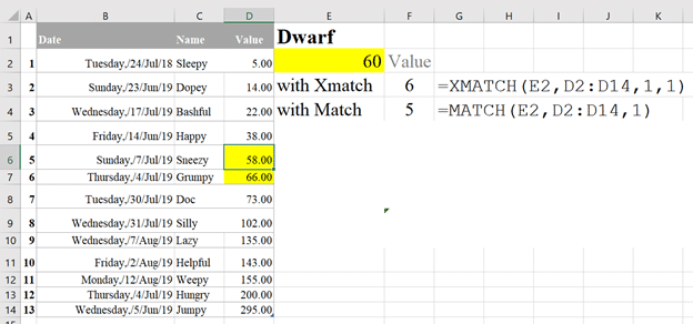
As soon as ascending data is placed in the list, Match() will be able to calculate the value, which is in the 5th position (next smallest match).
XMatch() is definitely the more refined and usable function in Excel. It can work with both horizontal and vertical ranges. Match() will always return the first match within the array, whilst XMatch() provides added search behaviors to enhance your searches, such as the reverse search.
Xlookup is coming and it’s truly a great thing
Xlookup now available for all Excel 365 platforms
New and better features in Office 2021 and Office LTSC