Our Year Planner Excel workbook download is just the start. Here are many suggestions for changes to improve or customize the download. Tips for changing the headings, overall look, change financial year, highlight public holidays, change the look of a day in the week, change weekend shading or day label.
We’ll even show how to change the day of week labels to another language including Klingon!
Some of these ideas come from our readers while others are answers to readers questions. To start you’ll need the Yearly Planner / Calendar for Office Watch readers
Headings
Many readers had very different opinions about the column headings (top row) or month labels (left column). They all suggested different changes depending on their personal taste.
Here’s some ideas you can use:
Change row height
Change the height of the top row by dragging.

If you’d like more space between the numbers and the January row, change the vertical alignment to Top. That will leave space below the digits. Or use Bottom align for a closer fit.
It looks screwy to us but Trevor J. from Wisconsin likes the Home | Alignment | Angle Counterclockwise look to angle the day numbers.

Another approach from Ron S. is to add a spacing row and column. Then it’s easy to adjust the spacing or reformat the ‘blank’ row/column.

Wider columns
Wider columns let you fit in more text, make a bigger planner or have larger day labels.
Before changing the column widths get the current width. Select a single column, right-click, choose Column Width and make a note of the value.
Now select all day columns (B to AF), right-click then Column Width. Most likely the value will be blank, that’s why we suggested getting the single column width first. Enter a larger value for width.
Change look
We added cell styles to make it easy to change the overall look. There are four cell styles:

Day Cell Default – the formatting of each day before conditional formatting kicks in.
Day Number – the top row 1
Month Name – the left column A
The last, all black, style is ‘No Day’ for the end-of-month cells. The formatting hides the name.
Change any of the styles to quickly change the overall look.
The weekend shading and formatting for 29th Feb (Cell AD3) is in Conditional Formatting.

An annoyance in Excel is that conditional formatting has to be done manually. It’s not possible to apply a cell style name to a conditional format.
Format as Table
The entire Year Planner can be converted into an Excel Table. Some readers like this, we’re not so sure there’s any great advantage.
Select the entire planner and choose Home | Format as Table.
Most likely you’ll want to turn off the Filter Buttons which will clutter up the top row
Banded Rows have no effect because there are cell styles and conditional formatting overlaying the table formatting.

Public Holidays and other special events
Any public or personal holidays are individually formatted either with a cell style or manual formatting.
We added cell styles for Public Holidays and Personal / Vacations.

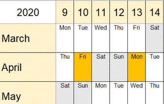
Unfortunately, the cell formatting only applies to weekdays. Conditional formatting for weekend days overrides other formatting (in other words, conditional formatting is applied last). This is Easter 2020 with 10-13 April all using the Public Holidays style but only Good Friday and Easter Monday show that style.
The workaround would be a more complicated conditional formatting formula. The formula would have to test the cell fill color and, sadly, that’s not possible with in-built functions like Cell(). Custom VBA or a legacy function would be necessary to get the fill property.
Fixed date holidays can be manually formatted because the date cell remains the same for any year.

Christmas Day will always be cell Z13 (unless you’ve added more rows/columns).
4th July cell E8
Australia Day AA2
Highlight a day of the week
We were asked how to highlight a certain day (Tuesday) because it’s garbage day.
Add a conditional format like this:
=WEEKDAY(DATE($A$1,MONTH($A2),B$1),2)=2
Change the last digit to which day of the week you like. Monday = 1, Tuesday = 2 etc.

We’ve dug into the Format options Fill | Fill Effects to demonstrate another way to decorate a cell with a gradient option.
Block out past dates
The first Conditional Formatting rule can block out any dates before today with a simple formula.
=B2<Today() — B2 is the 1st January

The rule applies to all day cells e.g. =$B$2:$AF$13
Choose whatever formatting you like but make sure this rule is first, before the weekend and other rules.
Hide Year List
The pull-down list of years is sourced from the Year List tab/worksheet. For the sake of tidiness, you can hide it by right-clicking on the tab then Hide.

Or, bypass the need for the tab at all. An alternative is just typing a comma separated list of the years in the Data Validation for cell A1.

Better highlighting row and column
If you’re using the Year Planner in Excel (i.e. not printed) you might prefer different highlighting of the selected row or column. See Excel tricks to highlight selected row, column, heading and more
Change ‘weekend’ cells
There are two ways to change the conditional formatting that shades day cells as ‘weekend’.

The current formula is …
=WEEKDAY(DATE($A$1,MONTH($A2),B$1),2)>5
Weekday() returns a number for the day of the week. Saturday is 6, Sunday is 7.
The last two characters ‘>5’ is how Excel ‘knows’ it’s a weekend day. Change that part of the formula to alter the days shaded as weekend.
To shade just Sunday use:
=WEEKDAY(DATE($A$1,MONTH($A2),B$1),2)>6
or
=WEEKDAY(DATE($A$1,MONTH($A2),B$1),2)=7
Weekday() options
The alternative is changing the way Weekday() works. In the conditional formula, look for the , 2 parameter. That controls how Weekday() numbers the days.

Change the setting to ,1 as in
=WEEKDAY(DATE($A$1,MONTH($A2),B$1),1)>5
will shade Friday and Saturday.

Day of Week label
Using a custom cell format ‘ddd’ to get the day of the week is the most elegant method but there are other options that are more explicit with options.
Instead of a Custom cell format, you can apply the formatting within a formula with the Text() function. Text() converts a value into another format using the same formatting codes that Custom formatting does.
=TEXT(DATE($A$1,MONTH($A2),B$1),"ddd")
That’s really another way of doing the same thing. Some people might prefer it because the formatting of the days is more obvious in the formula.
Another language
Maybe you’d prefer to show the days in another language from Excel’s default. That’s possible using a combination of Weekday() and Choose()
=CHOOSE(WEEKDAY(DATE($A$1,MONTH($A2),B$1)),"Sun","Mon","Tue","Wed","Thu","Fri","Sat")

Now you can change each of the day labels like this for French, Chinese and Klingon.
=CHOOSE(WEEKDAY(DATE($A$1,MONTH($A2),B$1)),"Dim","Lun","Mar","Mer","Jeu","Ven","Sam") =CHOOSE(WEEKDAY(DATE($A$1,MONTH($A2),B$1))," 星期天","星期一","星期二","星期三","星期四","星期五","星期六") =CHOOSE(WEEKDAY(DATE($A$1,MONTH($A2),B$1)),"wa","DaS","pov","ghIt","logh","buq","ghIn")
Yearly Planner / Calendar for Office Watch readers
Office Watch has extensive help to make Calendars in Word, Excel, PowerPoint and Outlook.