Excel can make bar charts in-cell without bothering with the full Chart system. Despite what you might have seen, there’s plenty of options in Excel Data Bars.
The usual example of Excel Data Bars has the colored bar in the same cell as the value. In this article we’ll show how it’s possible to have the data bar alone, showing percentages instead of values or a data bar which includes negative values in a different color.
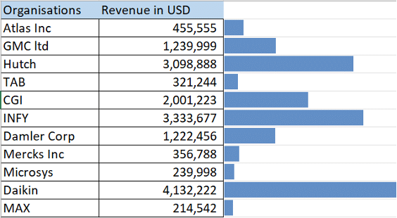

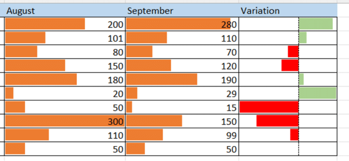
Excel Data Bars are an alternative to Building In-Cell Bar Charts in Excel.
Data Bars in Excel are an integrated form of conditional formatting that visually represents the values within cells by inserting colored bars. The length of each bar reflects the cell’s value in relation to others in the range, with longer bars indicating higher values and shorter bars representing lower ones. This makes it easy to spot trends instantly, for example the top and bottom-performing products in a sales report.
Before we continue, it’s important not to confuse data bars with bar charts. Bar charts are separate graphical elements that can be moved around the sheet, data bars are integrated into individual cells and remain fixed within them.

Add data bars in Excel
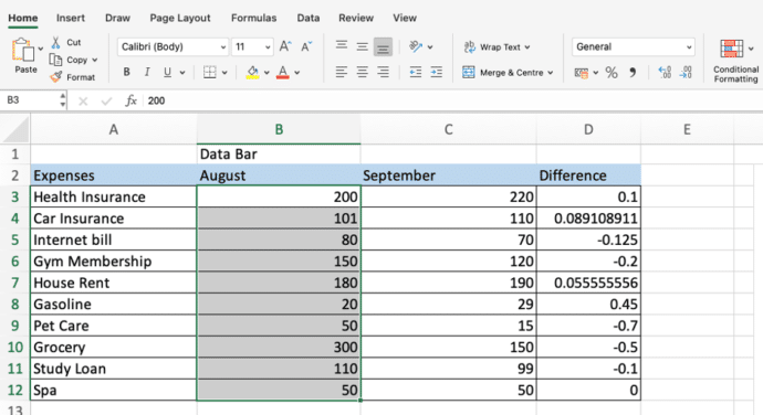
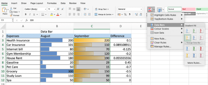
Launch the Excel spreadsheet where you want to apply data bars then highlight the range of cells where you want to insert the data bars. Navigate to the Home Tab |Conditional Formatting under the Styles group.
Hover over Data Bars and select the style you prefer, either Gradient Fill or Solid Fill. Once selected, coloured bars will automatically display within the chosen cells.
The below screenshot shows how to apply Solid fill.
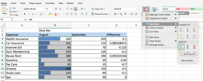
To insert Gradient fill data bars in Excel, select your preferred color under the Gradient Fill option:
Customising Data Bars
Do not get dishearten if the available preset formats do not meet your requirements, you can create a custom rule with your own data bar style.
Select the cells where you want to apply data bars. Then, navigate to Conditional Formatting | Data Bars |More Rules.
In the New Formatting Rule dialog box, customise the options as per your choice.
Select the data type for the Minimum and Maximum values. The default option (Automatic) typically works well, but you can choose alternatives like Percent, Number, or Formula if you want more grip over how the values are calculated.

Set the Bar direction to either context (default), left-to-right, or right-to-left.
Show Data Bar only
If you prefer to display only the colored bars without the cell values, check the “Show Bar Only” option. Adjust the Fill and Border colors until you’re satisfied with the preview.

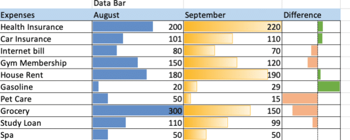
Click OK and you get your customised data bars with a custom gradient color, using all other default settings.
Excel data bars based on another cell value
When using preset conditional formatting, there isn’t a straightforward method to format specific cells based on the values in other cells. This can be particularly useful when applying data bars with very bright or dark colors, which may obscure the cell values.
Fortunately, there is a simple workaround for this issue. Copy the values to a new set of cells then apply conditional formatting with only the data bars showing.
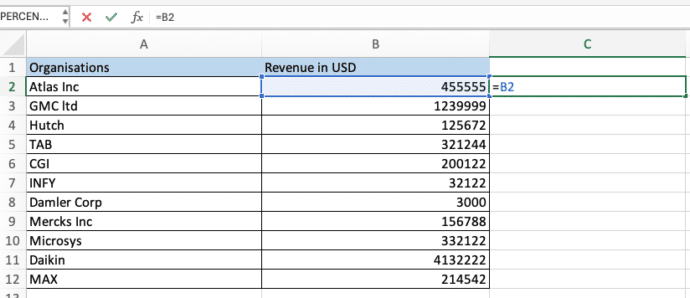
Copy the original values into an empty column where you want the data bars to appear. To ensure the copied values remain linked to the original data, use a formula like = B2, assuming B2 is the topmost cell containing your numbers.
Next, apply data bars to the column where you’ve copied the values. Navigate to Conditional Formatting | Data Bars |More Rules and in the Formatting Rule dialog box, select the “Show Bar Only” option to hide the numbers. And that’s it!
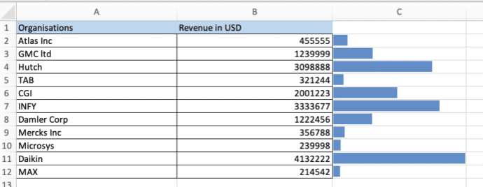
For example, if the numbers are in column B, you would use the formula =B2 in cell C3 and copy it down the column. As a result, you’ll have the numbers in column B and data bars in column C.
Define minimum and maximum data bars value
When using preset data bars, Excel automatically determines the minimum and maximum values. However, you have the choice to customize how these values are calculated.
If you are creating a new rule, navigate to Conditional Formatting | Data Bars |More Rules.
For editing an existing rule, navigate to Conditional Formatting | Manage Rule. In the list of rules, select your Data Bar rule, and click Edit Rule.

In the rule dialog box, under the “Edit the Rule Description” section, select the desired options for the Minimum and Maximum values that you prefer. When done, click OK.
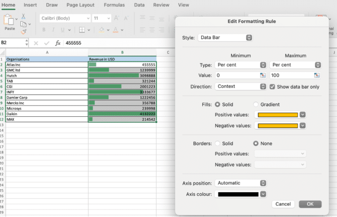
For instance, you can set the data bar percentage with the minimum value at 0% and the maximum value at 100%. This way, the bar representing the highest value will fill the entire cell, while no bar will appear for the lowest value.
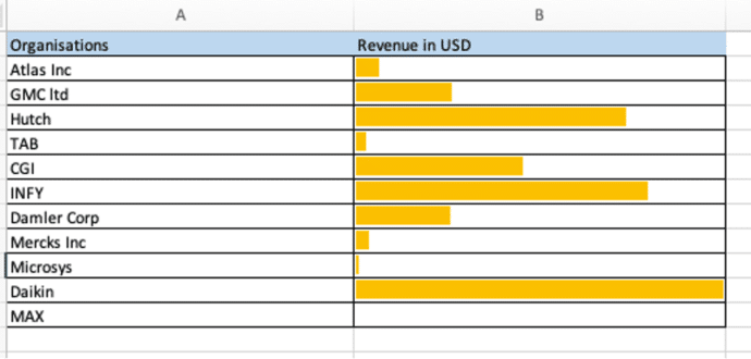
Excel Data bars for negative values
If your dataset includes both positive and negative numbers, you’ll be pleased to know that Excel data bars also accommodate different bar colors for positive and negative numbers.
In the New Formatting Rule window, under Bar Appearance, select the color for the positive data bars and negative data bars.
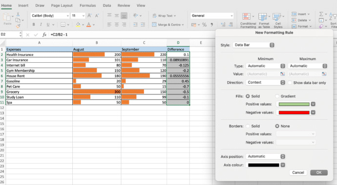
Click OK to close the windows and apply your colours to the data bar.
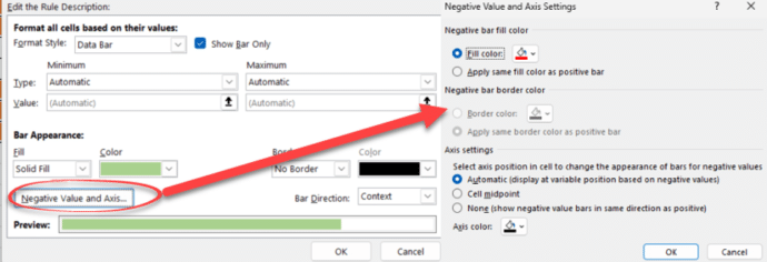
In Windows, choose “Negative Value and Axis Settings” to see the options for negative fill color, border color and Axis settings.
Now, you can easily spot negative numbers with a quick glance at your dataset.

Building In-Cell Bar Charts in Excel
Excel Conditional Formatting, beyond the presets
Excel is getting better Conditional Formatting with much needed improvements