Excel List in a Cell: One Cell Now Holds Many Values, but Don’t Share It Yet

Excel cells can now hold a list of values instead of just one, a major change in how Excel behaves. A single cell can store several names, dates or times that formulas treat as separate items. It’s in preview for Microsoft 365 Insiders on Windows and Mac only, so for most people the advice is simple: try it on a copy, and don’t send workbooks with list cells to anyone until Microsoft explains how other versions of Excel, Google Sheets and data tools will handle them.

At its simplest, a list cell is a dynamic array or list compressed into a single cell instead of being spread across many cells.  One of Microsoft’s examples is listing split times for runners. There’s a new icon at the left of the cell followed by a list of the times.

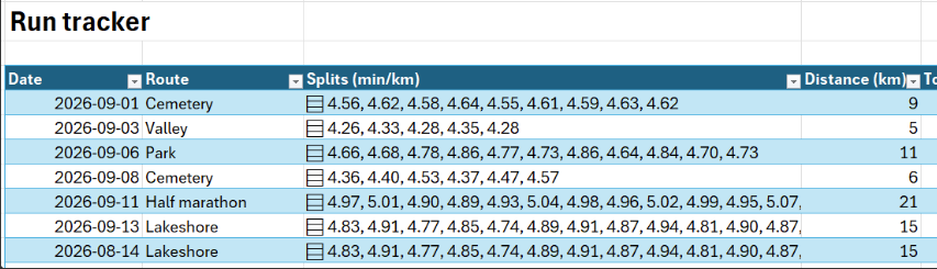
Before lists in cells, each split time would have to be in a separate cell. Now they can be put into a single cell but handled like a group of cells.

This feature is very new and, for the moment, only for Insiders on Excel 365 for Windows or Mac.  However, it’s a major change in how Excel can work, which will eventually be available to all Microsoft 365 customers, so it’s worth a close look.

List cells are genuinely useful, and arguably the biggest change to how Excel cells work since dynamic arrays. Arrays in cells and especially nested arrays are power user territory. They can be hard to follow and debug, and may slow down large workbooks.

How to make a list in a cell

Use Insert | List or press Ctrl+J, then type or paste items separated by commas or semicolons.

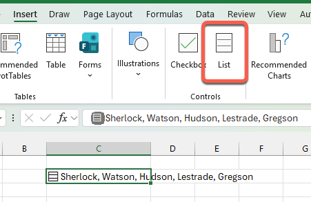
Just like Linked Data Types, there’s a Show Data Type Card on the right-click menu or click the little icon at left of the cell.

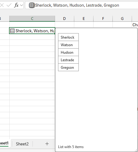
A few practical points:

• Ctrl+J is a toggle. Press it again and the list turns back into plain text.
• Editing works as normal. Double click or press F2.

Referencing a list cell returns a spill or dynamic array

If you reference a list cell, you’ll get a dynamic array of the list elements.

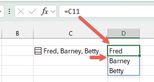
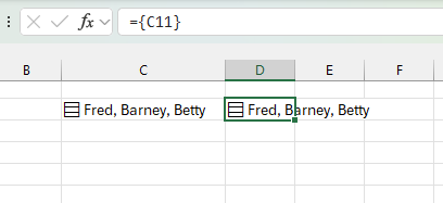
To get a copy of the list cell, add curly brackets around the cell reference, for example ={C11}.

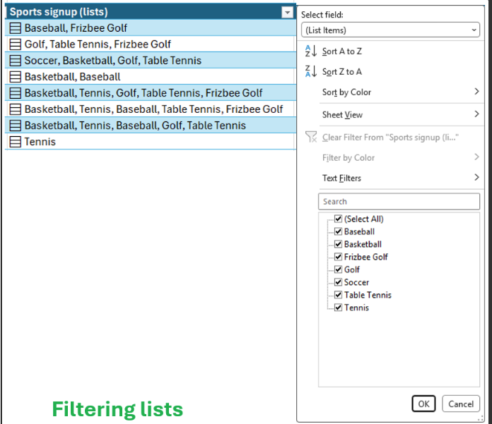
Filters get smarter with list cells

Once a column holds lists, the filter dropdown shows each list item once rather than every full text string.

Keeping formula results in one cell

The second part of the feature is arrays in cells. Normally a formula like SORT or FILTER “spills” its results down the sheet. Typing a curly brace right after the equals sign and another at the very end, like ={SORT(B3)}, keeps the whole result in one cell.

This is especially handy inside Excel tables, where a spilling formula normally fails with a #SPILL! error.

Don’t confuse these with old array formulas

The new braces are just typed normally and go inside, right after the equals sign. The old Ctrl+Shift+Enter braces sat outside the formula and Excel added them for you.

How long a list can be?

Microsoft hasn’t said how long a list array can be, so we did some tests.

The longest list we could make hit Excel’s maximum of 32,767 characters per cell.

The big concern is how Excel handles the overflow, at least for now. Any text over Excel’s limit is silently cut off without an error, so be careful pasting a long list into a single cell.

Four new functions to work with lists

Microsoft added four functions to work with lists:

Has() functions

The three Has() functions let you search inside a list.

HAS() checks whether one value is in a list, for example =HAS(A2,”Bob”). It matches whole items, so “Bob” won’t match “Bobby” or “Bobbie”.

HASALL() returns TRUE only when every value you give it is in the list. It’s useful for questions like ‘show me projects where both Ann and Bob are involved.’

HASANY() returns TRUE when at least one of your values is in the list.

Flatten()

FLATTEN() breaks lists apart so each item gets its own cell.

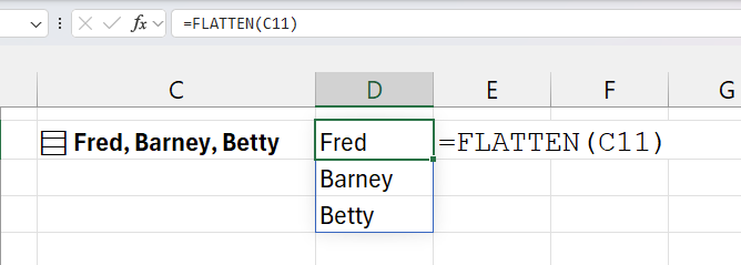
Wrapping it as =SORT(UNIQUE(FLATTEN(<list cell>))) gives you a clean sorted list of every item with duplicates removed.

Your existing favorites work too. COUNTA, SUM, SORT, UNIQUE, XLOOKUP and GROUPBY all work with the items inside a list.

Other functions like LEN() return a dynamic array with the length of each item in the list.  To get the character length of the whole list use =SUM(Len(<list cell>)).

Is a cell a list?

It’s easy for a user to tell if a cell contains a list: just look for the little icon at left.

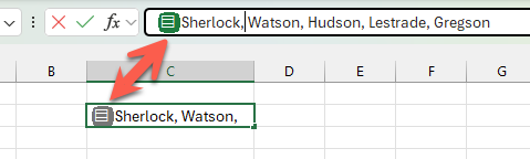
Programmatically though, there’s no good answer. The Type() function will return 64, but that’s the same result as an array.  COUNTA() returns the number of items in a list, so it helps when the result is greater than 1. However, that’s no help when the list has only one item.

Microsoft needs to add a new value to the Type() function or make an IsList() function.

What characters are list separators?

Microsoft hasn’t explained which characters can be used as list separators. The official demos use either commas or semi-colons and there are suggestions that the Windows/Mac regional setting applies.

We tested commas, semicolons, colons and the pipe character (|) as separators, and they all work.

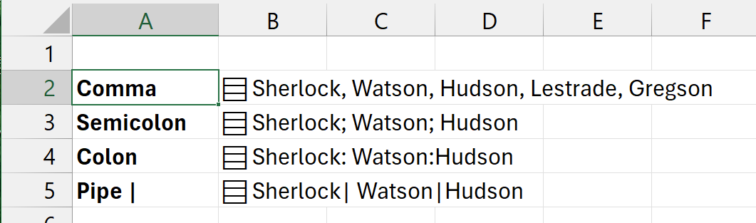
Just like other delimited lists, choose a separator that doesn’t conflict with the content. For example, if your list includes commas in the items, use another separator.

Nested arrays: arrays inside arrays

The most advanced piece is nested arrays: arrays that contain other arrays. Microsoft’s example is TEXTSPLIT: without nested arrays Excel only returns the first item for each row, but with them the full result comes back, one array per row. If you’ve ever tried TEXTSPLIT inside BYROW and got a #CALC! error, this is the fix.

Compatibility Version 3

Most nested array calculations need Compatibility Version 3, set per workbook under Formulas | Calculation Options. Microsoft admits some existing formulas return different results in Version 3, and says you can keep a workbook on Version 1 or 2 if it misbehaves.

In plain English: flipping that switch can change the answers your existing formulas give. Microsoft hasn’t listed which formulas are affected in a way most people can act on. Never change it on a live workbook. Test on a copy.

What doesn’t work yet

This is a preview, and it shows. Lists don’t yet work with PivotTables, charts, Power Query, data validation dropdowns (a list can’t be the dropdown source), Find & Replace on individual items, or conditional formatting unless you use a rule based on a formula.

For many office users, PivotTables and charts are the whole point of a spreadsheet. The workaround is to FLATTEN the lists into regular cells before a report uses them.

As mentioned earlier, Microsoft should add a reliable way to detect a list cell.  However, they didn’t bother to add a way to identify dynamic array or spilled data cells (except in VBA) so don’t hold out a lot of hope.

There’s sure to be other bugs arising from this major change in how Excel behaves.  That’s what beta testing is for, and we hope Microsoft won’t skimp on this important work in a rush to release publicly.

The sharing problem

This is where we’d be cautious. A list in a cell is a brand new kind of value, and the rest of the Excel world doesn’t understand it yet.

If you send a workbook full of lists to a client on any other version of Excel (regular Microsoft 365, Excel 2024, Excel 2021 and so on), a colleague on Google Sheets, or a finance system that reads the file automatically, you have no guarantee what they’ll see.

Don’t share workbooks with the new list cells unless you know the receivers also have the latest Insiders builds of Microsoft 365 desktop. Even then, make sure the other users understand list cells.

Microsoft hasn’t published how lists, arrays in cells and nested arrays will be stored in the .xlsx file. That affects apps that import Excel data with no concept of cells with multiple values, including CSV exports., Google Sheets, LibreOffice, and older Excel builds. Data tools that expect a cell to hold only text, a number, TRUE/FALSE or a date, such as the Python libraries openpyxl and pandas, may also need updating.

Who gets it?

The rollout is going to Microsoft 365 Insider Beta Channel users on Windows Version 2610 Build 20520.20000 or later and Mac Version 16.114 Build 26092111 or later. Only Windows and Mac have been announced, and because the rollout is gradual you might not see it even on the right build.

Dynamic Arrays, Spills and Smarter Excel

List cells are only in the Beta Channel for now, so before you switch, read Microsoft 365 Insiders: Is It Safe and Worth Joining? to find out what can go wrong and how to back out if a beta build misbehaves.

Lists in cells build directly on dynamic arrays. If you’re not sure your copy of Excel has them, Do you have Dynamic Arrays in Excel 365? shows a quick test, and Make any Excel function dynamic (almost) reveals how everyday functions like ROUND and TRIM can spill results too.

Once you FLATTEN a list, it plays nicely with Excel’s modern functions. Excel GroupBy Function Tutorial: A Complete Guide shows how to summarize data without a PivotTable, while Text Splitting Functions Excel you must try explains the TEXTSPLIT function that nested arrays finally fix.

Lists can’t feed a dropdown yet, but the workaround in Excel Drop-Down List from Dynamic Arrays gets you most of the way there. For clean, automatically updated lists, Live Sorting and Filtering in Excel Made Easy combines SORT and FILTER in one formula.

Curious about the old braces the new syntax replaces? Excel Array formulas for everyone explains the Ctrl+Shift+Enter method, and Understanding the new Lambda helper functions covers BYROW and friends if you want to push nested arrays further.