Array formulas are an important part of Excel and they are a lot more important now that dynamic array formulas are around. Don’t ignore arrays because they’re an unavoidable part of Excel for everyone.
This is the start of a series to help you understand arrays in Excel. At the very least, you’ll know what happening when upcoming Excel changes appear in your worksheets.
Arrays take a bit of understanding, but it’s worth it. They help make Excel faster and more streamlined.
At present, Excel supports ‘array formulas’ only when specifically setup. But Excel 365 for Windows is getting ‘dynamic array formulas‘ that are setup automatically.
Dynamic or Automatic arrays coming to Excel 365 for Windows
The current Excel needs you to explicitly make an array formula (using Ctrl + Shift + Enter, we’ll explain below).
Microsoft calls the new feature ‘dynamic’ arrays but we think of them as automatic arrays.
If you see a cell error like #SPILL. They happen when Excel thinks you want a dynamic array but you’re just using Excel the ‘old fashioned’ way. It means the cell result is an array but there’s not enough empty cells (usually down a column) to fit the results.
What is an array?
Anyone who did Programming 101 can skip this section <g>.
An array is just the nerd name for a list or grid of values – the values can be anything, it doesn’t matter. All these columns are separate one-dimensional arrays of different values.
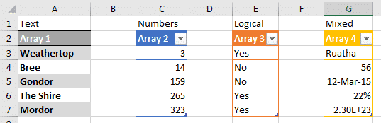
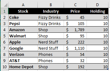
Arrays can get more complicated. This is a simple two-dimensional array, aka a grid or table.
Arrays can go into three or more dimensions but let’s not go there … it starts getting mind-boggling.
Excel arrays don’t exist in cells or tables. They are made in memory, temporarily, for calculating the result. That’s faster than making more cells and columns.
Array formulas
We’re used to Excel formulas that work off individual cells. Array formulas work with a range or list of values. We’ll start with simple array formulas that make an array and give a single result.
Advanced array formulas give the result as an array. We’ll get to that in a later article.
A simple array formula at work
Let’s start with a simple table, sales figures for two months and a comparison of the two in column D.
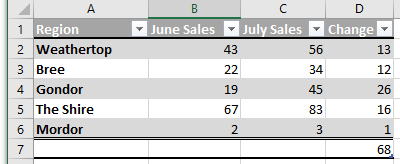
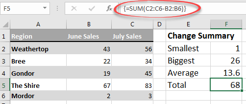
With array formulas, we don’t really need the ‘Change’ column D at all. Array formulas can combine all that detail in a single formula line. Here’s a sales change summary without the Change column.
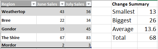
We’ve jumped straight from the sales figures to MIN, MAX, Average and SUM summaries without the middle step.
Here’s the SUM array formula:
{=SUM(C2:C6-B2:B6)}
Notice the curly brackets around the entire formula? That indicates an array formula.
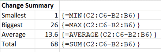
Here’s all the array formulas. The same array using different Excel functions:
Under the hood
With the cell reference: C2:C6-B2:B6 Excel has subtracted each of the cell pairs.
To see that, select the array part of the formula and press F9
=SUM({13;12;26;16;1})
That reveals the array of numbers in the cell references. In this case, the digits are the same as in the old ‘Change’ column D from the first screen shot above.
Making an array formula
What makes the difference is the shortcut: Ctrl + Shift + Enter (Command + Return on a Mac). That makes an array formula instead of a regular formula.
An array formula is the same as a regular formula except you type Ctrl + Shift + Enter to complete the formula.
Important: An array formula appears with the curly braces except when editing. The braces disappear when you edit the formula which is very annoying and a trap.
More Important: you must type Ctrl + Shift + Enter every time you edit the array formula. If you accidentally type Enter, it’ll become a regular formula again.
Don’t type the curly brackets/braces … only Ctrl + Shift + Enter adds the array formula braces.