Everyone knows the SUM function in Excel but that’s just the start, there are eight SUM() functions (and more) for adding up numbers in different ways.
SUM()
SUM is one of the first functions taught to newcomers. It’s as old as Excel itself (older because SUM was in the first spreadsheet program, Visicalc)
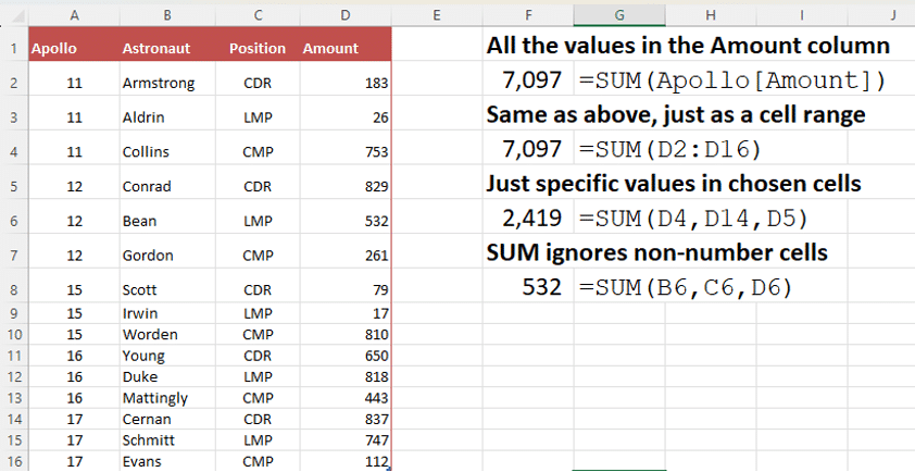
In its simplest form, give a range of cells to add up:
SUM(D2:D37) – adds up all the values in cells D2 to D37.
SUM(Salaries) – adds up all the values in the named range ‘Salaries’
SUM(Payroll[Amount]) – adds up all the values in the column ‘Amount’ in the table ‘Payroll’
More than one value can be separately chosen like this:
SUM(A2, D7, E8, F22, G1:G7) – adds up the values in those four cells and a range.
Non-number cells are ignored.
Here’s SUM at work with a table of values.
Space Nerd Note: to keep the list small for demo purposes, only the moon landing Apollo missions are listed. No disrespect meant to the other Apollo astronauts and especially not to the crew of Apollo 1.
SUBTOTAL()
Subtotal() is a function mostly used with tables and groups but it has two useful properties that makes it worth mentioning as an alternative to SUM().
Subtotal() totals up the currently filtered table, not the entire table.
It also has the option to include or exclude manually hidden cells.
Despite its name, SubTotal() can do other things to a range of numbers like Average, Count, Max, Min etc.
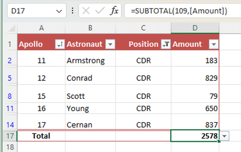
SUBTOTAL(function_num,ref1,[ref2],…)
The first parameter of Subtotal() tells Excel what calculation you want with two options for each, including or excluding manually hidden cells.
The code numbers for SUM in Subtotal() are:
9 – SUM with hidden rows
109 – SUM without hidden rows.
Subtotal() only includes rows that are filtered from a table, unlike SUM() which includes the entire table range regardless of the current filter. In this example, Subtotal() is only adding up the filtered rows (CDR or Commander only) not the entire table.
The second and later parameters are ranges to include in the Subtotal calculation.
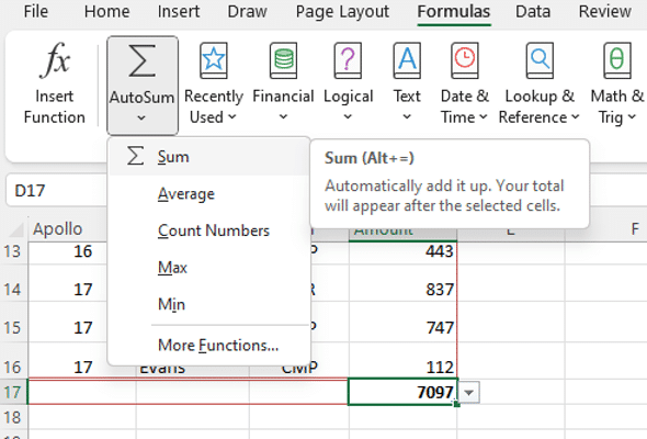
AutoSUM
A special case of SUM is Formulas | AutoSum or Home | AutoSum. Select the cells at the end of a column/s or row/s, Autosum will automatically add a Sum() or Subtotal() .
Make VERY sure that Autosum selects all the cells you need and none you don’t want added. A text or blank cell can stop Autosum short of a full list of values.
Shortcut: Alt + =
SUMIF()
SUMIF() is a filtered SUM, adding up only the values that meet a criteria.
There are two forms of SUMIF().
- Using the same list of values to both filter and add up
- Use a different criteria to filter, then add up another value from a matching row.
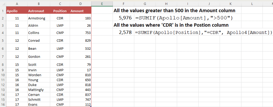
Here’s both SUMIF’s at work. First filtering by the Amount (only values less than 500) and then using the Position column to add up only the ‘CDR’ Amounts.
SUMIF(range, filter, [sum_range])
- range range of cells that you want evaluated by criteria.
- filter . Filter or crteria in the form of a number, expression, a cell reference, text, or a function that defines which cells will be added.
- Any text criteria or any criteria that includes logical or mathematical symbols must be enclosed in double quotation marks (“).
- Wildcards accepted – question mark (?) to match a single character, asterisk (*) to match any sequence of characters. To find an actual question mark or asterisk, add a tilde (~) before the character.
- sum_range Optional. The cells to add up, if you want to add cells other than those specified in the range argument, Sum_range should be the same size and shape as range.
Tip: Instead of SUMIF, always use SUMIFS because it’s easier to add more criteria later.
SUMIFS()
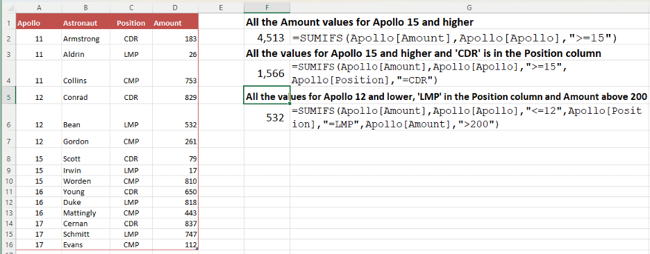
SUMIFS() solves a problem with SUMIF which can only handle a single criteria.
SUMIFS() accepts many separate filters in pairs of range plus criteria like this …
SUMIFS(sum_range, criteria_range1, criteria1, [criteria_range2, criteria2], …)
SUMPRODUCT()
SumProduct is a great shortcut when you need to multiply numbers together then add up all the results for a grand total. Most common use is multiply a price/cost with the number of units for each of a series of items. For example, the total value of items on hand.
=SUMPRODUCT(array1, [array2], [array3], …)
Without SumProduct, you’d have to make a separate column/row of the combined value of each item, then SUM() all those calculations into a grand total.

Product is another math word for multiply, a term I vaguely remember from high school.
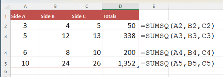
SUMSQ()
SumSq() squares each number then adds them together.
SUMSQ(number1, [number2], …)
Each parameter can be a cell reference or an array.
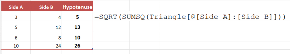
Could be called the Pythagoras function, because, combined with the SQRT() (Square Root) function, you can calculate the long side (hypotenuse) of any right-angle triangle.
Rules that apply to all these SUM functions
All these Excel SUMming functions have the same rules for their parameters, except SubTotal()
- Can be a mix of constants, names, arrays, or references with numbers.
- Ignored are empty cells, logical values, and text values when they appear in arrays or references.
Two more rules let you force values into the function by hardcoding or typing values into the function.
- Numbers hardcoded as text (like “1”, “7”) are evaluated as values, but only when they are hardcoded as arguments.
- Logical values TRUE and FALSE are evaluated as 1 and 0 respectively only when they are hardcoded as arguments.
DSUM()
Is a little like SUMIFS but the filters are in cells of a table with headings that match the source table.
In these examples we’re using the table A1:D15, adding up values in the ‘Amount’ column, filtered with the settings in the table F1:I3. First, just add up the Apollo 11 amounts (filtered by the ‘11’ in G2).

Here’s another with two filters in cells G2 (12) and H2 (LMP)
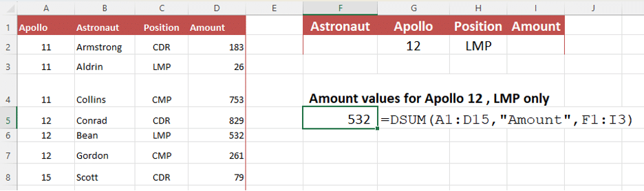
Note: the filter table headings must match the source table headings but not necessarily in the same order and not all the headings have to be shown.
The criteria heading and filter cells can be a named range.
Syntax
DSUM(Table/List, field, criteria)
- Table/List The range of cells that makes up the list or table, Microsoft calls it a database. The first row of the list contains labels for each column.
- Field Indicates which column is added up . Either the column label or a number that represents the position of the column within the list.
- Criteria The range of cells that contains the conditions or filters.
But wait, there’s more!
There are even more SUM related functions but these are obscure and more complicated. For the sake of completeness …
SUMXMY2()
SUMX2PY2()
SUMX2MY2()
These three functions compares the sums of two arrays.
SERIESSUM()
Calculates the sum of a power series.
IMSUM()
One for the math or Excel nerds who understand complex numbers. “Returns the sum of two or more complex numbers in x + yi or x + yj text format.”