Learn how to use Excel’s powerful SWITCH function, the modern alternative to nested IF statements. The SWITCH function evaluates a value against multiple matched outcomes and returns the first corresponding result, plus an optional default if nothing matches. Our guide breaks down the format, best usage patterns and practical examples plus tips for combining SWITCH with other functions for smarter, more compact logic.
The SWITCH() function finally solves a long-standing problem in Excel, making a essily understood set of nested IF statements. It’s a clean, modern way to simplify complex logic and keep your formulas readable.
Switch() is Excel’s version of a CASE statement in other languages and with a little trickery also IF ELSE. It lets you evaluate one expression against multiple values and return a corresponding result, without stacking long IF or IFS formulas.
As a bonus I’ll show how to use Choose() with Switch().
Excel 365, Excel 2019 and later plus the browser-based Excel all have Switch().
Using the SWITCH() function
It’s a compact, self-contained lookup when you have several possible outcomes. If none of the values match, SWITCH can return an optional default result.
The structure of the SWITCH function is as follows:
=SWITCH(expression,val1/result1,[val2/result2],...,[default])The first argument, called the expression, can be a constant, a cell reference, or a formula whose output will be tested. Each matching value must be followed by its corresponding result, and SWITCH can process up to 126 such value–result pairs. A final optional argument lets you specify what to return when no match is found.
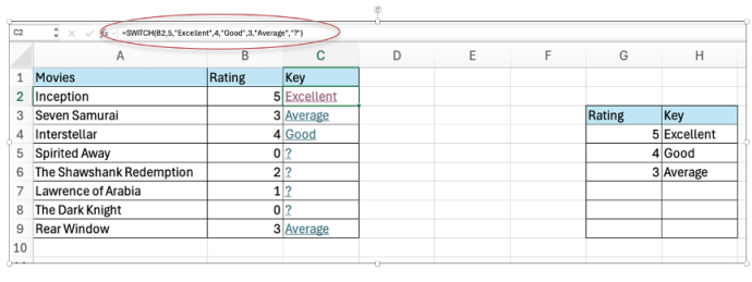
Let’s look at a rating example where SWITCH creates a cleaner formula.
=SWITCH(B2,5,"Excellent",4,"Good",3,"Average","?”)Here, B2 (rating or score) is matched against specific numeric ratings, and the corresponding label is returned.
Using different tests within Switch()
Officially SWITCH can only check for exact matches (like a CASE statement) however there’s hidden depths available.
In practice, each Switch() test (the 2nd, 4th etc parameter) has to return TRUE or FALSE. Use that to add any test you like into Switch.
Use logical operators like greater than > or less than (<) etc directly like this common workaround is to make SWITCH test for TRUE, then put formula into each parameter like this:
=SWITCH(TRUE, A1>=90, "Excellent", A1>=75, "Good", A1>=50, "Average", "Dumb")This assigns a performance label based on the score in A1. Again, while SWITCH can do this with the TRUE workaround, IFS () is typically more natural for comparison-based conditions.
The order of Switch() tests is important because Excel will return the first TRUE statement it reaches and ignore the rest.
Use SWITCH when you want a clean, simple alternative to nested IF statements and when outcomes depend on exact matches or a small set of conditions.
Example of SWITCH with Dates Excel Functions
To understand how SWITCH works alongside other functions, imagine you have a list of dates and want to quickly identify whether each one is today, tomorrow, or yesterday. In this case, you can use the TODAY() function, which returns the current date’s serial number, together with the DAYS() function, which calculates the number of days between two dates. Combining these with SWITCH allows you to classify each date at a glance.
You can see how well SWITCH handles direct value-to-label mapping.
=SWITCH(DAYS(A2, TODAY()), 0, "Today",1, "Tomorrow", -1, "Yesterday", "Unknown")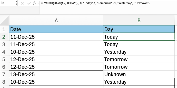
DAYS(A2, TODAY()) compares the date to today. SWITCH maps the number to a text label.
Using CHOOSE ()
AlthoughSWITCHandCHOOSEare different functions, they solve similar problems:
they both return a result based on a single input. But they do it in different ways.
CHOOSE() selects a value from a list based on a numeric index (1 = first item, 2 = second, etc.)
=CHOOSE(2,"Red","Blue","Green") returns Blue
CHOOSE only works with numbers, not text conditions or logical tests. It’s available in Excel 365, Excel 2016 and later.
SWITCH + CHOOSE Together (Powerful Combo)
You give CHOOSE a number (1, 2, 3, etc.), and it picks the corresponding item from a list. While SWITCH is great for matching exact values or labels, CHOOSE is best when your choices are arranged in a numbered order. When used together, SWITCH convert conditions into a number and CHOOSE returns a result based on that number—making your formulas cleaner and easier to maintain.
Let’s say you want to grade scores into A, B, C, or Fail by using the SWITCH function to determine the correct category based on score ranges and then using CHOOSE to return the corresponding grade label.
Formula =CHOOSE(SWITCH(TRUE, A2>=90, 1, A2>=75, 2, A2>=60, 3, 4), “A”, “B”, “C”, “Fail”)
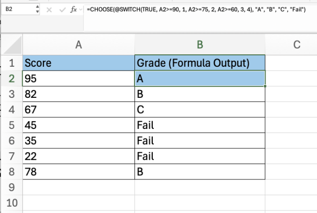
What SWITCH(TRUE, …) does is evaluates each condition in sequence—if the score is 90 or above, it returns 1; if it’s 75 or above, it returns 2; if it’s 60 or above, it returns 3; and if none of these conditions are met, it returns 4.
CHOOSE() uses this returned number to pick the appropriate grade from the list “A”, “B”, “C”, and “Fail”. For example, if A2 contains 82, SWITCH returns 2, so CHOOSE outputs “B.”