Filter is another Excel 365 dynamic array formula that’s really useful and far better than similar options in earlier versions of Excel.
Just like SORT() and SORTBY(), FILTER() refreshes automatically whenever the source values change. The older pull-down filter and sort choices don’t update properly. Dynamic Arrays also give you the choice to show the same data in different orders or filters at the same time.
Here’s a simple FILTER() example with source data of exam results.
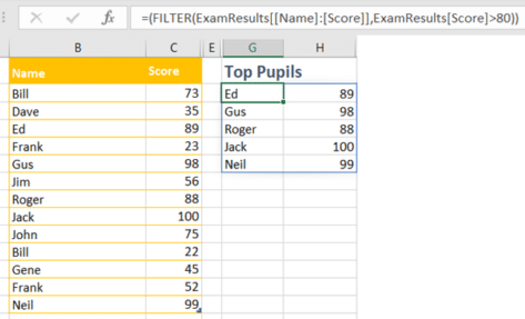
On the left is the source data, a boring old Excel Table cunningly labelled ‘ExamResults’.
On the right is a list of the pupils who scored more than 80, created with a basic Filter() formula.
Filter() is available in Excel 365 for all platforms, Windows and Mac, Apple, Android and Online. Also the upcoming Excel 2021 and Excel LTSC.
Automatic updating
A quick example of why Filter() is better than the table pull-down filtering.
Let’s say the exam results are revised (re-marked by another teacher, parent complaints, accusations of cheating, more pupils added from a make-up exam, even name typos). Here’s the revised results.
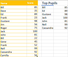
The ‘Top Pupils’ list at right has automatically updated results and names. It adds newly qualifying pupils and drops others. No need to refilter from table pull-down commands, no risk of outdated information being displayed, Excel 365 does it all
Inside Filter() options
The syntax for Filter() is simple with two necessary parameters and a third optional which is highly recommended.
=FILTER(array,include,[if_empty])
Array
Required (obviously)
A table, array or range you want to filter from.
Include
Required (naturally)
The test to apply as a filter. The test has to return either True or False for each row, just like a test in other formulas like IF()
IF Empty
Optional, but important
What to display if there’s no results to the Filter(), can be any value including text.
Separating Source from Results
As we’ve already mentioned, dynamic arrays need a change in the way Excel users think about arranging their worksheets. Until now the broad concept was to show the source table then use the pull-down selectors to sort and filter that list.
With dynamic arrays the source data is separated from the displayed lists. The source could be hidden altogether, especially if it’s imported via PowerQuery.
Here’s what you can do with Filter() to ‘slice n dice’ the original list in different ways – all visible at the same time with no pull-down selectors necessary. The top, failing, passing and really bad pupils all appear in separate lists.

If nothing for a Filter()
The right-most column shows the handy final parameter of Filter(). You can specify a value or text string to return when there’s no results from the filter.
In this case, there’s no results below 10 so the list shows ‘None’.
That’s a more elegant feature than forcing the user to make a clumsy IF statement to handle the ‘no result’ exception.
It’s IMPORTANT to include the third parameter if there’s any chance of a ‘no result’ Filter(). Excel doesn’t like empty results and will show a nasty #CALC error if not told what to do.
Better live sorting in Excel 365
Dynamic Arrays now in Excel for iPhone and iPad
Excel now has Dynamic Arrays – Windows, Mac and more …