Excel’s PivotTable allows you to evaluate trends, comparisons, and patterns within datasets. Once a PivotTable is setup, you can filter “Drill down” into it to focus on key information.
These days there are several ways to filter a PivotTable, Slicers (which Microsoft loves to boast about), AutoFilter and by Field List.
All these options mean you can start with a (relatively) large data source, knowing it can be narrowed down within the PivotTable.
Our ebook! PivotTables and PivotCharts from scratch, for Microsoft Excel
PivotTable in Excel
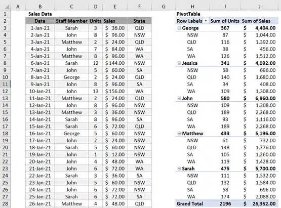
First, you will need to build your PivotTable. If you have any trouble in creating PivotTables, check out make your first PivotTable in Excel.
We have created a PivotTable to the right using the large dataset at left.
Filter Data with the Slicer Tool
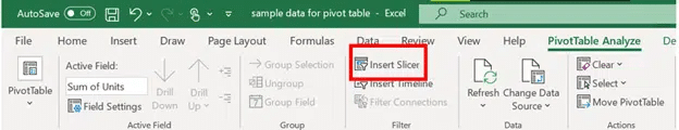
Select any cell within the PivotTable, then select PivotTable Analyze | Filter | Insert Slicer
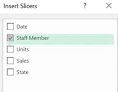
Select the fields you wish to create slicers for and select OK.
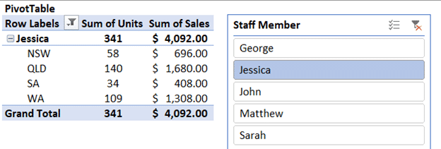
Excel will show the Slicer Table which you can move and adjust according to your liking.
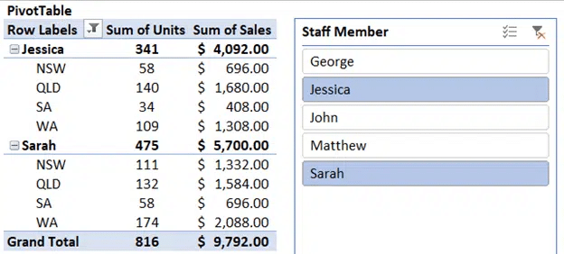
Select a slicer check box to filter the PivotTable. In this example, we have chosen Staff Member, but you can select more than one. That shows all the available choices (Staff Members in our example) as separate buttons.
You can hold down Ctrl and click buttons to select more than one button to Filter.
AutoFilter Data
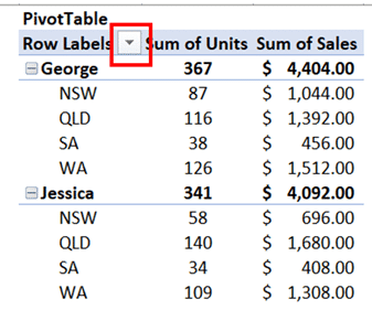
By selecting the drop-down arrow under Row Labels, you can filter the data to your preferences.
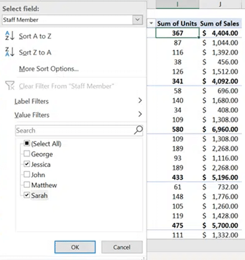
Just untick (Select All) to deselect all boxes, then manually tick the boxes of data you wish to show.
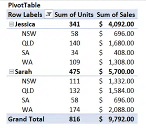
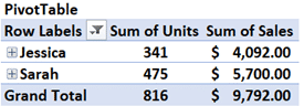
In the example below, we will tick data for Jessica and Sarah.
You can also select the minus and plus buttons to expand or collapse the breakdown of information.
AutoFilters will work with slicers, so you can create a high-level filter with a slicer before diving deeper with AutoFilter.
Filtering by Field List
Filters can be added to the PivotTable’s Filter field.
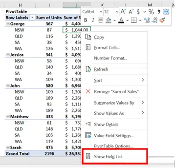
Simply right click anywhere within the PivotTable and Select Show Field List.
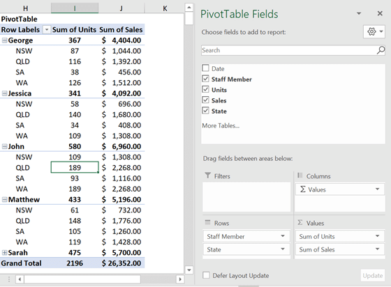
If we wanted to filter the data by State, we can select and drag State from the Rows box into the Filters Box.
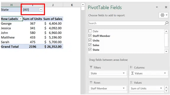
Excel will adjust the PivotTable with All State data.
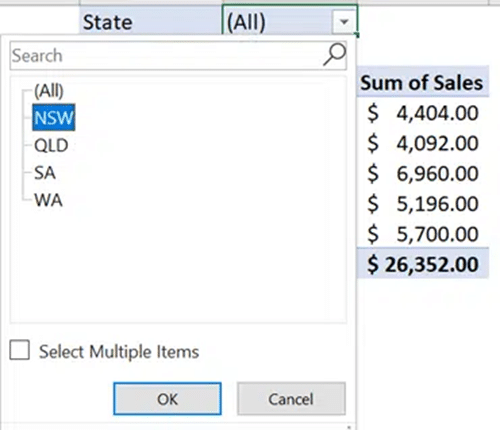
Select the drop-down box next to State, select the State you wish to filter and press OK.
If you wish to select more than one State, tick the Select Multiple Items box
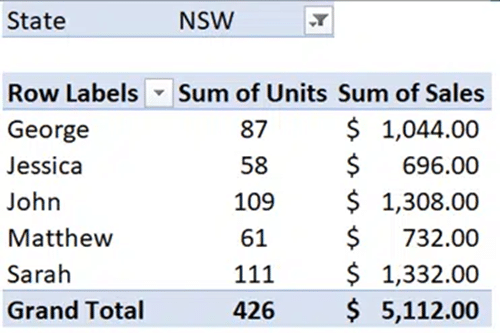
We have filtered the PivotTable by NSW below:
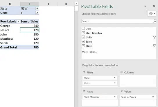
You can select multiple fields to Filter, for example being able to Filter by State and Units.
Great ebook! PivotTables and PivotCharts from scratch, for Microsoft Excel
Faster PivotTables with the new Ideas or Insights feature in Excel
Excel Slicers beyond PivotTables into Tables
Timelines for date filtering Excel PivotTables