There are two ways to hide Excel cell contents that you don’t want visible, but still available able to use in calculations. It’s another case of Office having an official and unofficial hiding option.
Here we’re talking about hiding individual cells or ranges. There are separate options for hiding row, columns or entire worksheets (aka tabs).
Hiding cell formulas – according to the manual
The approved method is part of Excel’s Protection racket feature. It hides cell formulas but NOT the results. That’s handy if you’re sharing a finished workbook.
Select one or more cells, right-click and choose Format Cells … then the Protection tab. Or press Control + 1 shortcut.
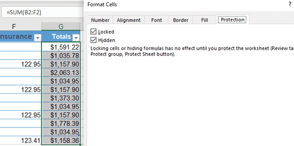
Choose the Hidden option.
As the text note on the tab says, marking a cell as ‘Hidden’ doesn’t hide it. ‘Hidden’ means ‘hiding formulas’.
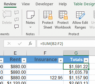
Truly hide the select ‘Protect Sheet’ or ‘Protect Workbook’ on the Review tab. The password is optional.
Once Protected, any ‘Hidden’ cells will hide the formulas.
See the Formula bar is now blank for all ‘Hidden’ cells.
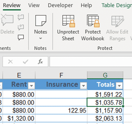
To reveal the formulas again, click Unprotect Sheet.
Unofficial hiding cells with cell formatting
The other hiding option completely blanks out the cell – formula and value.
To do this, just select the cell(s) you want to hide and either:
- Press Control+1, or
- Right-click and select Format Cells.

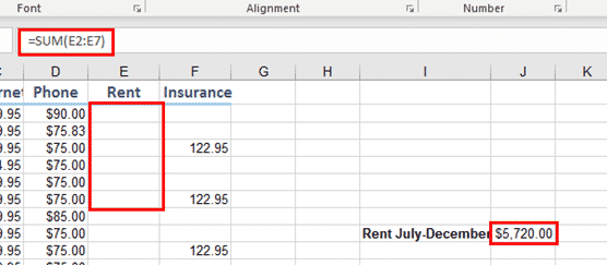
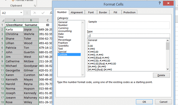
In the Format Cells dialog, we select the Number tab, and select Custom at the bottom of the list. In the Type field, we type three semi-colons (;;;).

The figures in those cells are now invisible, but they can still be used in formulas.
Why Semi-Colons?
Why is this seemingly random string of characters is used to hide cell contents. Well, it’s not random at all! The semi-colons come from the way that custom number formats are structured in Excel. If you look at the formats already listed in the Type field of the Format Cells dialog, you will see a bunch of strange symbols. We won’t go into the details of how these work in this article, but the important thing to notice is that they all have semi-colons interspersed in them.

What is happening here is that these symbols are telling Excel how to display four different types of data, and the types are separated by semi-colons:
<positive-values>;<negative-values>;<zero-values>;<text-values>
Whatever you put in each of those positions signifies how to display that type of value. If you want everything in that cell to not be displayed, you simply leave them all blank, leaving you with just the three semi-colons.
Showing Hidden Cell Contents
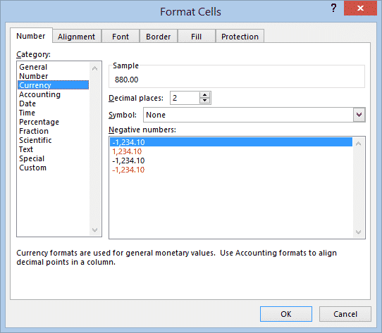
If you have hidden some cell contents and later decide that you need to view them again, it is very easy to display them. Simply select the cells again and open the Format Cells dialog (Control+1 or right-click + Format Cells). Back on the Number tab again, we just choose the appropriate category for the type of numbers we are displaying (in this case, Currency).
Hiding Text Content
You can do exactly the same thing on text cells, and the data will still be hidden.

Hiding isn’t deleting
A reminder that hidden data isn’t deleted. Anyone with access to the worksheet can see the original data. That’s important whenever data privacy is a consideration.
Why you must use the Document Inspector
Secrets left in docs after Document Inspector in Office