A list with groupings (like Product Type, Country, Region or Staff pay level) can become a nested PivotTable. The sub-totals are created with + – signs to show/hide the groupings.
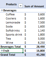
We’re using the same source list as in our Basic PivotTable and Two-dimensional PivotTable examples.
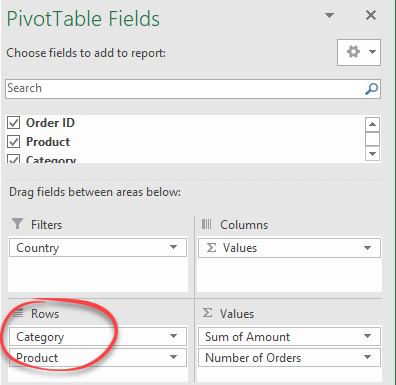
Doing that is simple, just drag a second item down to the Rows area:
Drill down more
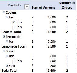
Adding another row level lets you drill down even more. In this case to the date of each order.
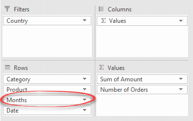
Adding a date field will automatically group as well, in this case by Month. You can drill down from the top level (Category) to sales by month and finally sales per day.
If you don’t want the auto-grouping just choose the Remove Field option from the pull-down menu for the grouping eg ‘Months’.