There’s a nice little Excel function that will calculate the rate of return on any asset like a stock or fund including income/dividends with purchases and sales over time. The secret sauce is XIRR() a function which calculates an internal rate of return with uneven interest or dividend payments. In other words, common real-world situations.
There are two other functions IRR() and MIRR() which give a rate of return for unchanging payment situations like a simple fixed interest bond.
XIRR() can handle more complex and realistic situations like returns on a stock or mutual fund where the dividends can change dates and values over time. Also, occasional purchases and sales of shares.
Office-Watch.com will go beyond the usual XIRR examples to show how the function is used in the real world.
Use XIRR for many things!
XIRR has many uses for any asset where you want to work out the return, either capital or income.
Stocks, shares, mutual funds even an investment property all work with XIRR()
The only exceptions are fixed interest securities and that’s only because IRR() might be a better and easier choice.
Where is XIRR()??
XIRR() is a quite old Excel function. It’s in all Excel for Windows from Excel 365, Excel 2021/2019 back to Excel 2003.
Excel for Mac from Excel 365, Excel 2021/2019 back to Excel 2011. Also in Excel on the web.
A really simple XIRR()
Let’s start with a simple example of XIRR, just to see how it works. An investment of $10,000 on 1 June 2015, $1,000 interest is paid a year later on 31 May 2016 with the principal repaid the same day.

Obviously, that’s a 10% return. Now see how the rate of return increases a little if the same interest is paid in two instalments.

XIRR – Yearly rate of return
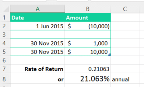
XIRR gives a yearly percentage rate of return, here’s the same values as the last example but over only 6 months. The rate of return has roughly doubled because the date range halved.
XIRR syntax and rules
At its core, XIRR is quite simple to use. A list of values with a matching list of dates is all that’s needed. Plus an optional rough guess of the answer to get the calculation started.
Formally it XIRR looks like this:
XIRR(values, dates, [guess])
Values The cash flows, starting with the initial investment as a negative number. Investments are negative values while any returns (interest, dividends, sale of the asset) are positive values.
Dates The dates that each value occurred to match the values list. Dates have to be in Excel serial form (make sure they aren’t text).
Guess is optional and defaults to 10% (0.1) but can be vital. It’s a number that you think is close to the result of XIRR. See “The XIRR guess is important” below.
RETURNS: an annual rate of return as a percentage i.e a 10% return is 0.1.
XIRR notes
- Remember that XIRR returns a percentage, for example a 12% return is given as a value of 0.12 . Use the Percentage cell format. In our examples we’ve shown both the raw value and the nicely formatted percentage.
- XIRR is quite tolerant of empty rows and just ignores them.
- Serial dates are used in XIRR, any time of day element (i.e to the right of the decimal point) is ignored.
- Dates can be in any order.
- There must be at least one positive and one negative value.
The XIRR guess is important
The guess value can be important because Microsoft has limited XIRR to 100 tries or iterations. If it can’t get a result after 100 tries, XIRR returns a #NUM error.
If you’re getting a #NUM error using XIRR, one possible reason is the guess. Trying adding a reasonable guess value if the possible result is very high or very low.
The guess only has to be very roughly correct. The default is 10% or 0.1 in these days of low returns 0.01 (1%) might be necessary.
In theory, a more accurate guess allows Excel to run faster (i.e fewer iterations), but it’s unlikely to make a difference unless you have many, many XIRR functions in a workbook.
Calculate the return on stocks or shares in Excel
Let’s look at a practical example of Excel’s XIRR() can calculate the return on a stock, share or fund investment. We’ll explain how XIRR() works in the real world showing a return with or without capital adjustment.
This is a stock bought for $25,000 with varying dividends paid over the next two years.

XIRR shows a negative return! And a mighty large loss at that. That’s because we’ve not included the current value of the investment, as if it had been sold today or the last day of the reporting period (e.g. financial year or quarter).
Dividend and Capital rate of return
Adding the value of the stock today, the rate of return makes sense and includes the increase in stock value over two years.

Dividend only return
If you wanted to calculate the return from dividends only (no capital gain/loss) insert the original cost again but as a positive value and with today’s date (or end of the reporting period).

Separate columns for capital and income transactions
Normally, you’d have separate columns for capital and income transactions however XIRR can’t cope with multiple columns of values. The workaround is to make an extra column that combines the values from Capital and Income ranges into a single range that XIRR can understand.
The Combined column is the sum of the Capital and Income cells in that row. The whole column can be hidden to keep your worksheet tidy.
Here’s the same ‘Dividend only’ worksheet as above, but in a different form. Separate capital and income columns plus a Combined column (SUM of Capital and Income columns, per row) for XIRR to use.

Three new performance boosts for Excel 365
Excel 4 macros are now blocked and about time too
Excel Sheet View solves a collaboration problem
Fast stock charting with Excel and StockHistory()