To make data entry simpler in Excel, form controls such as checkboxes can be added. A checkbox can be used to select or deselect an option. Checkboxes are useful for forms that have multiple options.
The trick is using Excel’s Developer tab which holds the checkbox control. See How to get the Developer Tab in Office apps
Insert a Checkbox in Excel
Select the Developer Tab | Controls | Insert | Form Controls | Checkbox

Drag your mouse over the cell of your choice or select a cell within the worksheet.

A checkbox will appear, which you can use your mouse to move and adjust accordingly.
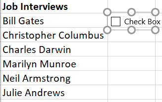
Change the Check Box Text
Simply right click the checkbox and select Edit Text

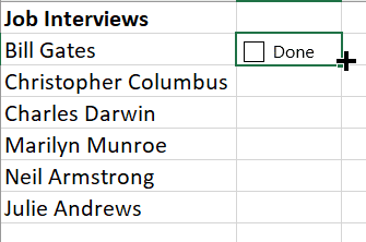
This will allow you to edit the text as preferred, you can also completely delete the text if you wish to have the checkbox only.
Copy the Checkboxes
To copy the checkboxes over to other cells, simply hover the mouse in the bottom right corner of the current cell until a cross appears.
Drag the cross to copy over to the other cells.


Copying individual checkboxes? You can right-click on the checkbox and select copy or Ctrl + C, then right-click another cell and select paste or Ctrl + V.

Once you select the checkbox, the box will automatically be ticked.
Format a Control
Formatting is important to allow you to customize the properties or appearance of your checkbox and linking a cell to a checkbox.
To format, right-click on your checkbox and select Format Control…

You can modify the following options in the Format Control Tab:
Checked: displays the checkbox that has been checked.
Unchecked: displays the checkbox that has been unchecked.
Mixed: displays a checkbox with shading which specifies a combination of cleared and checked states.
3-D Shading: Provides a 3-D look to your checkbox.
Here’s all the check box appearance options:

Cell Link
Under Cell Link: select the cell where your checkbox is located, in this example we have selected $B$2.
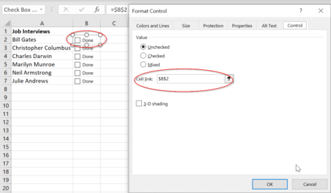
Now in the linked cells, it will appear as FALSE for unticked checkboxes, and TRUE for ticked checkboxes.

The TRUE and FALSE can then be used towards Excel Formulas and to adjust the formatting. As you can see, that text overlays the checkbox text we set above so if you use this option, you’ll probably not have any control text.
To hide the TRUE and FALSE when you check/uncheck the boxes, simply select the cell and change the text colour to white.

Unfortunately, with this Format, Excel doesn’t have a way to easily copy this to the other cells and automatically link the correct cell to the correct checkbox. We’ve even tried to use Format Painter but alas… you will have to action this manually for each individual checkbox.
Below we have actioned the next checkbox under $B$3.

Conditional Formatting
Next, we can apply conditional formatting so that when a box has been ticked, the text in another cell is marked accordingly.
Conditional Formatting works for a neighbouring or related cell but NOT the checkbox itself.
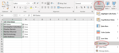
Select your list, in this example, we have selected A2:A7.
Go to the Home Tab | Styles Group | Conditional Formatting | New Rule
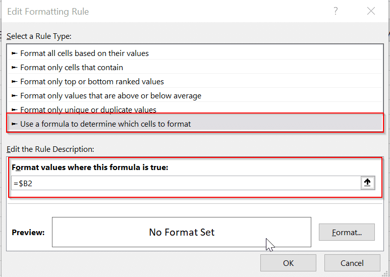
From the list, select Use a formula to determine which cells to format
Under Edit the Rule Description: place the first cell from your list, to ensure this is dynamic and will be applied to the other cells within Column B, we have removed the $ sign after B, =$B2
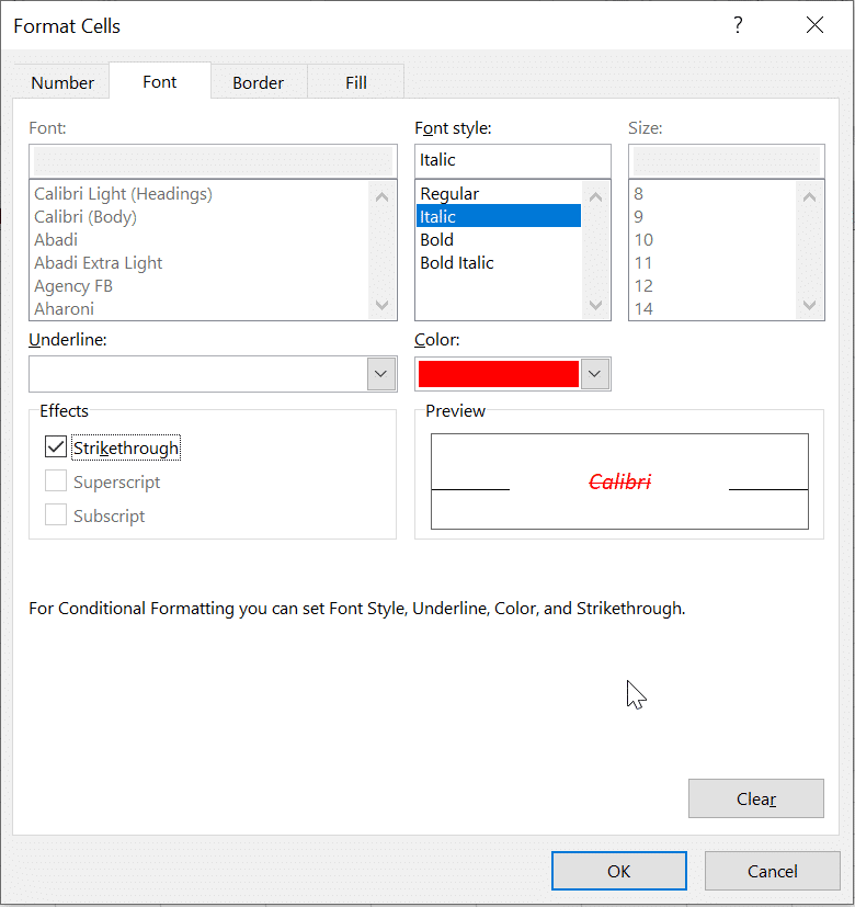
Then select Format… and adjust your Font settings. For conditional formatting you can change the Font style, colour, strikethrough, and underline.
In our example, we have selected Strikethrough, Italic font, and the colour red.
Once you have formatted to your liking, click OK.
Now the formatting will be applied to all boxes checked.

Get more from Excel Check boxes
See Clever ways to use Checkboxes in Excel
How to protect Excel sheets from unwanted changes – Part 1
The danger still lurking in Excel and how to stop it