Making unique (not duplicated) list in Excel is possible in three ways that update automatically. One is headspinningly hard. One has some minor quibbles. The best option is a lot easier and relatively new in Excel.
We’re talking here about making a list of unique (non-duplicate) values which update automatically if the source list changes. There is a ‘unique’ option table filtering option but it’s a ‘one off’ action that doesn’t refresh.
Why bother?
A surprising question about making a unique list is why it’s even necessary. After all, the question goes, “We know the list of departments, regions etc”, just type them in and move on.
Unique lists in Excel have many uses. In Totals or Summaries. Also making pull-down lists.
There are two main reasons why it’s better to produce unique lists that automatically update from the original data.
Expand or Contract automatically
If the list of stores, regions etc change an automatic list of unique values will update automatically.
Let’s say one of the seven dwarves has gone walkabout, the new automatically made list of values removes ‘Doc’ automatically (left).

Or maybe there’s a new (and very popular) dwarf added, it appears in the list without changing a single formula (right).
Error Checking
Automatic unique lists also quickly show data errors in the source list, like spelling mistakes:

A manually typed list (looking for a hardcoded ‘Bashful’) would ignore the misspelled item, making the totals and summaries incorrect. The auto generated unique list always shows all unique names, including spelling mistakes.
IFERROR with Index, Match and Countif
There’s a complex array formula that was made in the dim, dark past of Excel and passed down from developer to developer. An Excel meme, if you will.
It’s complicated but widely supported across Excel releases and past versions. You should not have to worry about compatibility as long as Excel supports array formulas (which have been around for many years)
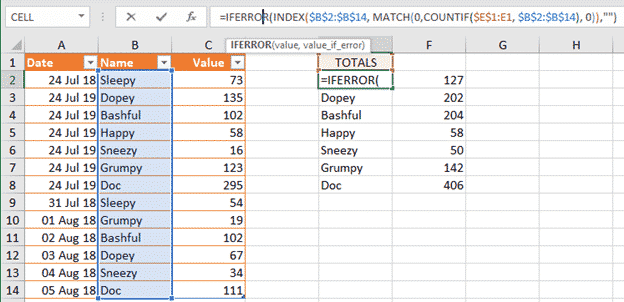
=IFERROR(INDEX(<range to search>, MATCH(0,COUNTIF(<absolute cell reference of cell at top of current column>:<current cell less one row>, <range to search – same as earlier in formula), 0)),"")Here’s the array formula in action making a list of all the dwarves in the list at left.
Far easier to copy and paste one of these formula (one with a table reference) then change the parameters to suit.
=IFERROR(INDEX($B$2:$B$14, MATCH(0,COUNTIF($E$1:E1, $B$2:$B$14), 0)),"")=IFERROR(INDEX(ShortPeople[Name], MATCH(0,COUNTIF($E$1:E1, ShortPeople[Name]), 0)),"")ARRAY FORMULA! This is an array formula, meaning the results spill into other cells. Keep clear the cells below the main cell with the formula.
The new Dynamic Arrays are NOT needed but you must end typing the formula by pressing Ctrl + Shift + Enter instead of just Enter. Ctrl + Shift + Enter tells Excel to make an array formula.
Using PowerQuery
A sneaky way to get a unique list of values is with PowerQuery. Normally PowerQuery is used to get data from outside sources before massaging it ready for an Excel worksheet.
PowerQuery can accept an existing Excel table as a data source. Then use PowerQuery’s options to make a unique list and drop the result back into the worksheet as another table.
This works quite well but isn’t available across all current Excel releases. It’s especially useful if you’re importing data from outside sources or using PowerQuery to do other things with the same data anyway. PowerQuery has other tricks available like automatic sorting, ignoring blanks and even replacing values.
The downside is recalculation. Unlike other Unique options, this PowerQuery trick does NOT update automatically, not even if you press F9. PowerQuery works on its own updating schedule.
It’s something we explain and workaround in our book Real Time Excel (because it’s very important for stock price updating).
First, click in a cell of the source table you want to use. Then Data | Get Data | From Other Sources | From Table/Range.

Because the cursor is in a table already, Excel assumes that’s the table you want to import and does it right away.
Removing duplicates couldn’t be easier. Select the column you want to de-duplicate then PowerQuery Home | Remove Rows | Remove Duplicates.

Then select the other columns and choose Remove Columns.

Now you have a simple list of unique names. Close and Load inserts a new table into Excel. Feel free to move that table to a better location, like next to the source table.

Another issue with the PowerQuery method is this incorrect warning when opening the workbook.

Security Warning: External Data Connections have been disabled.
Of course, there aren’t any external connections. The only connection is internal (i.e from a table in the current workbook).
Click ‘Enable Content’ then the prompt to make the workbook a Trusted Document. That will stop those prompts in future.
The new and better way Unique()
Here’s the super-simple way to make a unique list of names. It’s so easy you’ll wonder why it hasn’t been in Excel for years.
The new Dynamic Arrays feature includes a simple, direct version of the IFERROR… etc. formula mentioned above. UNIQUE() does all the work and some more.
Dynamic Arrays are in Excel 365 across all platforms.
All that’s needed is a source list like the name of a table column. Mostly, the two optional parameters aren’t needed.
=UNIQUE(ShortMen[Name])
Simple as that. The results will expand or contract automatically and recalculate any time the source list changes.
The sub-totals column F uses SumIF()
The full function is:
Unique(<range>, <by column>, <occurs once>)Range
the source list of names/values. The documentation talks about an ‘array’, in this contest any range or table reference is enough/
by_column
[optional] how to sort the list. The default is FALSE for row; by column = TRUE.
Clarification: the FALSE default means looking down a column which is usual (i.e the range has the same Column reference but different rows B2:B23) . TRUE means a horizontal array working across (the range has different letters B2:F2).
occurs_once
[optional] the default is FALSE – all unique values, TRUE = values that occur once.
FALSE gives a list of all the values in the list, no matter how many times each name/value appears (left).
TRUE shows only names that appear once (right), any name that appears more than once is ignored.

Comparing the occurs_once FALSE (left – showing all names) with TRUE (right – showing only names that appear once)
Unique() makes a once difficult task really easy in Excel
Using Unique() to make an Excel drop-down list
PowerQuery mystery – how to Remove Duplicates, keeping most recent record
Match and Index lookup in Excel