There are several ways for an Excel table to be transposed (rows and columns) but none of the online suggestions work very well with tables. We’ve found a solution which transposes one table into a ‘swapped’ table i.e headers become column A and column A becomes the headers.
Along the way we’ll explain a clever use of Power Query, how to run VBA code when certain cells are changed and how to refresh all or a single query from VBA. If you’ve not used PowerQuery, this is a simple, useful and self-contained starter.
This is what we’re trying to do. At top is a list of exam results from the town of Bedrock and a page right out of history.

The bottom table is transposed so we can filter / sort by subjects instead of students.
What’s needed is a way to take a source table and make a transposed version which is also a table AND updates automatically whenever the source changes. There are many times this kind of transposed table is useful yet it’s not truly and properly supported even in modern Excel.
The transpose solutions that aren’t good enough
Microsoft, among many, offers two Transpose methods, neither are truly what’s needed.
Paste | Paste Special Transpose
is OK but is a ‘once-only’ action not suitable for changing source data. And it doesn’t work for whole tables.

Transpose()
The Transpose() function would seem ideal because it works from a source Excel table.
BUT, the result isn’t an Excel table and can’t be converted into a table (because Transpose() returns a dynamic array).
Transpose an Excel table into another Excel table
The trick is to use Power Query which has its own Transpose function which, with a little tweak, will do what we need AND drop a full Excel table back into the worksheet.
Sadly the updating from changed source data isn’t automatic but there’s a VBA fix for that if you need real-time updating.
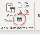
Select the source table then Data | Get & Transform Data | from Table

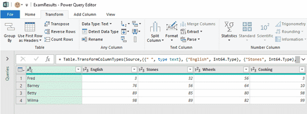
That imports the current table into the Power Query editor.

Power Query has a Transform | Transpose option but it will remove the existing headers (not move them to rows). Before Transposing, convert the headers into a normal table row (this is the ‘little tweak’ we mentioned)
Go to Transform | Use First Row as Headers | Use Headers as First Row

Now the table headings are in row 1.

Choose Transform | Transpose to swap the rows and columns.

Finally use Transform | Use First Row as Headers to convert the new top row into headers.

One of the many great things about Power Query is that it’s all recorded as a series of steps that are repeated each time the data is refreshed.

Close and Load the query into your worksheet. By default, the new transposed table is dropped into a new sheet. We moved it to the same sheet as the original table.

Two tables, the original (top) and the transposed (bottom) each with its own table filters and other Excel table goodies.
Make sure you only edit the original/source table. Any changes to the second table will be overwritten when the data is next refreshed.
Delinking the tables for fixed data
If your source data is fixed (like exam results) then you can just delete the query. Its transpose trickery won’t be needed again. Right-click on the query in the Queries and Connections pane then Delete.

The second transposed table will remain but delinked from the original table.
Updating the query and table
Let’s suppose the original table has values that will change over time. Maybe Fred & Barney will complain that their wives did better?
There are a few options for updating the transposed table after the original table changes. Which one you choose depends on the situation.
Each query has some update options, right-click on a query then Properties | Usage.

Refresh every … minutes might be enough but it still means the two tables could be out of sync.
Refresh data when opening the file should be ON.
Refresh this connection on Refresh All should be ON.
None of these are good options because there will always be a time delay between changing the original table and the transposed table updated.
The real-time updating fix
The better fix is to force a query update whenever a cell in the source table is changed. For that we turn to VBA and one of its event handlers.
Excel VBA has an automatic trigger or event when there’s a change in a worksheet: Worksheet_Change(ByVal Target As Range) in that function you can add code to only work when certain cells in the worksheet are changed. The basic function looks like this:
Private Sub Worksheet_Change(ByVal Target As Range)

    Dim CellsChanged As Range

' CellsChanged is the cells that will trigger an action if changed.
‘ change to whatever range applies to the source table
    Set CellsChanged = Range("A1:E5")

If Not Application.Intersect(CellsChanged, Range(Target.Address)) Is Nothing Then

   ‘ do whatever you want here

End If  ‘ change in one of the CellsChanged range

End Sub
What we want to do is refresh the query which is simply this line:
ActiveWorkbook.RefreshAll
That’s the VBA equivalent of pressing Data | Refresh All.
Update a single query in VBA
Most workbooks will stick with RefreshAll but if there are a lot of queries in the workbook you might not want to refresh them all, to update a single query use:
ActiveWorkbook.Connections("Name_just_the_query").Refresh
NOTE: the query name is NOT the name that appears in PowerQuery and the Power Query editor, for VBA it must be prefixed with ‘Query – ‘. For example this query ‘ExamResults-transposed’

In VBA is called ‘Query – ExamResults-transposed’ as in:
ActiveWorkbook.Connections("Query - ExamResults-transposed").Refresh
No, we don’t understand it either, but that’s what works!
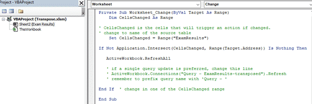
Full VBA update query on change code
The Worksheet_change function goes in the VBA for the sheet with the original / source table.

As a final little tweak the Range() is now the name of the source table, not a fixed cell reference. That lets the code work if the table is resized.
Private Sub Worksheet_Change(ByVal Target As Range)

    Dim CellsChanged As Range

' CellsChanged is the cells that will trigger an action if changed.
' change to name of the source table

    Set CellsChanged = Range("ExamResults")

If Not Application.Intersect(CellsChanged, Range(Target.Address)) Is Nothing Then

   ActiveWorkbook.RefreshAll

   ' if a single query update is preferred, change this line
   ' ActiveWorkbook.Connections("Query - ExamResults-transposed").Refresh
   ' remember to prefix query name with 'Query - '

End If  ' change in one of the CellsChanged range

End Sub
Make list of Excel sheets/tabs – automatic and even better
Three ways to understand part of an Excel formula
Excel single cell trick to get the latest stock or currency rate