Make it easier to see your current cell in an Excel workbook by dynamically highlighting the selected row, column, cell or headings. Here’s obvious and more subtle highlighting options plus the downside of highlighting, real world tips and debugging tricks if you’re having trouble.
There are many different variations on this method; two colors, headings only, cell only etc. We’ll also explain the workings so you can change the highlighting to suit yourself.
Large Excel tables can be hard to navigate and ensure you’ve selected the right cell. That’s especially important when you’re filling in the table gradually and in a random order – choosing the right cell is important.
We used this trick for a Trivia Quiz worksheet. Managing the scores with all the noise and confusion of an event can be difficult. This highlighting trick makes entering team scores more reliable.

Any modern Excel for Windows or Mac can do this. The Cell() function is essential and was introduced in Excel 2007 for Windows and Excel 2011 for Mac.
Dynamic highlighting by selection has two ingredients. Conditional formatting which uses the selected cell location as a condition plus a little VBA to make Excel do some extra work.
The magic ingredient – SelectionChange
The main trick is to make Excel recalculate the worksheet whenever you switch to another cell. Normally, Excel only recalculates when there’s a change in a cell or data refresh.
To do that, use a little VBA code to do something each time the selection changes. Excel has an in-built event for this called Worksheet_SelectionChange all we have to do is give that event something to do.

This code goes into each worksheet that you want it to work in.
Private Sub Worksheet_SelectionChange(ByVal Target As Range)
   If Application.CutCopyMode = False Then
      Application.Calculate
   End If
End Sub
The code invokes the SelectionChange event then forces Excel to recalculate the worksheet. We don’t want that to happen when we’re cut/copy/pasting so the IF statement stops that.
This little chunk of code has other uses, as you’ll see in the Headings of a selected cell option below.
Downside of forcing calculation
Forcing Excel to recalculate the worksheet for every cell movement will slow down the entire workbook. That’s true but probably not noticeable except for really large or complex worksheets. Modern Excel is pretty smart about figuring which cells to re-calc when a manual Calculate is done.
Give the highlighting a try, if it becomes a problem, just remove the VBA code or comment out the Application.Calculate line.
The workbook will have to be saved in a macro-enabled .XLSM format which can be an issue in some organizations.
The Conditional Formatting sauce
We’ve talked about Excel Conditional Formatting many times before. Usually it’s to change the look of a cell based on the value in that cell.
This time we’ll get sneaky. We’ll give Conditional Formatting a little formula that compares the currently selected cell location (row and column) with the cell to be formatted. If the cell is in the same row or column as the cell you’ve clicked in, the Conditional Formatting will be done. It’s an extension of an Office Watch trick applying conditional formatting to other cells.
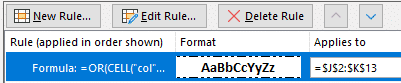
You can just copy/paste the formula below but if you understand how it works, it opens up a lot more possibilities. The alternatives we’ll look at below are mostly about changing this formula:
=OR(CELL("col")=COLUMN(),CELL("row")=ROW())
It’s not that scary, let’s break it down:
CELL("col")=COLUMN()
Compares the column number of selected cell CELL(“col”) with the column of the cell to be formatted COLUMN(), if they’re the same the result is TRUE
CELL("row")=ROW()
Compares the row number of selected cell CELL(“row”) with the row number of the cell to be formatted ROW(), if they’re the same the result is TRUE
Each of those tests returns a TRUE or FALSE, we want the formatting to apply when either case is True so both tests are wrapped in the OR function
The VBA code is necessary to make Excel recalculate the CELL() functions each time the selection changes.
Highlight selected row and column
Now let’s put all this together to make the row and column highlighting from the first image in this article. If you’re trying this for the first time, try this example first because it’s the basis for all the later variations. Get this one working and the rest will be a doddle.
Select the entire grid or table then Home | Conditional Formatting | New Rule.
Choose ‘Use a formula to determine which cells to format’.
Paste in the formula detailed above:
=OR(CELL("col")=COLUMN(),CELL("row")=ROW())
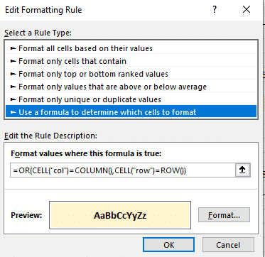
Then click Format to select the look you want. The Fill tab changes the cell background color.
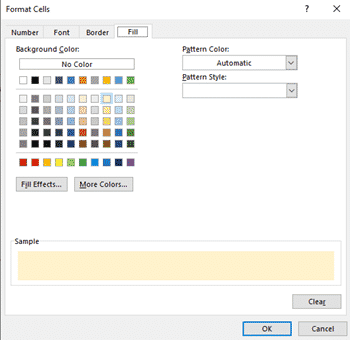
Border is also available to change the edges of the cell, there’s an example of that below.
Highlight row & column with different colors
Maybe you’d prefer the row and column to have different colors or formatting.
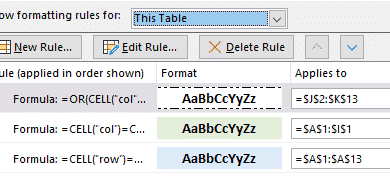
That’s just a variation with two conditional formatting rules, one for rows, the other for columns.
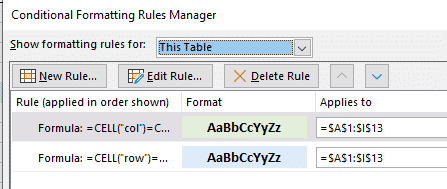
Both rules apply to the same range, grid or table.
Above we explained how the condition formula works, here are the two conditions:
=CELL("col")=COLUMN()

=CELL("row")=ROW()
As you can see, it’s the two tests without the OR() test to combine them.

Real World tip
It’s likely that you or users of the worksheet will ask for changes to the dynamic highlighting. Maybe a change of color or highlighting just rows etc. To make future changes easier, we suggest always setting two conditional formats (one for rows, one for columns). Even if both use the same formatting as in this example.

If the user/client wants a change, all you have to do is alter the formatting. For example, for row highlighting only, just clear the formatting options for the =Cell(“col”) … line.

Don’t delete the conditional formatting rule, you may need it again later!
More subtle, less obtrusive formatting
The above column and row formatting options are commonly demonstrated because they are obvious and showy. In many situations something more subtle is better.
Highlight the selected row or column only
The formatting for row and columns, shown above, is also the way to highlight just a row or column.

Use either the row or column conditional formatting.
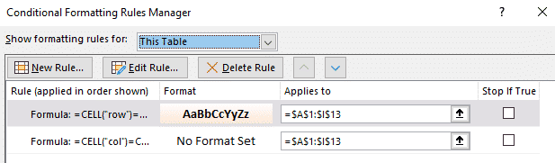
(we left the column conditional formatting in case we change our mind.)
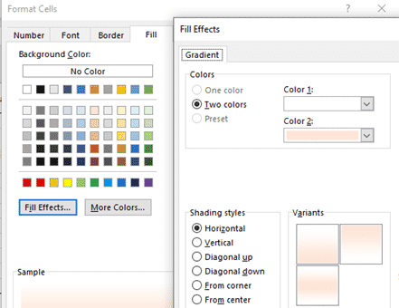
Cell gradient effect
The formatting is a two-tone gradient available at Format | Fill | Fill Effects | Two colors
Highlight headings of selected cell plus some extras
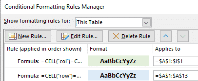
You might think the full colored lines are too much, how about highlighting just the row & column headings (Row 1 and Column A).

Change the ‘Applies to… ‘ to just the first row ($A$1:$I$1) or column ($A$1:$A$13).
Cell border formatting
The above example has few extra tricks, because we can’t help ourselves and have little fits of enthusiasm.
On the right side you’ll see Totals and Rank columns with top/bottom border edge formatting, just to show that alternative. That’s one of the options available on the Format Cells | Border tab.
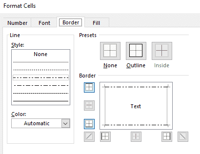
Instead of color fill, try horizontal and vertical borders to show the selected row/ column.
The conditional format only applies to those two columns.
Dynamic summary
The second trick is below the table and deserves an article of its own. It’s a summary of the selected student (row) that changes according to the cell you’re in.
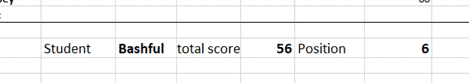
It’s an example of what’s possible once Excel is recalculating for each selection change. You can make more responsive and informative worksheets.
Do it with the INDIRECT() function which gets the value of another cell.
=INDIRECT(ADDRESS(CELL("row"),1))
Plus our old friend Cell() to get the selected cells row or column position.
Highlight just the selected cell
Even more subtle is highlighting just the selected cell. Excel does that automatically with a border around the selection but you can do more than that with conditional formatting. Here the selected cell is bold with yellow fill.

Do it with a simple variation on the very first formula at the start of this article.
=AND(CELL("col")=COLUMN(),CELL("row")=ROW())
Instead of OR() use AND() … meaning that both conditions have to be TRUE.

Debugging Tips
This trick has several steps and can be frustrating at first. Once you get it working, it’s great but that first try can drive you a little crazy. We’ve included some debugging tricks below.
Is the VBA working?
Make sure the VBA code is working by adding a message box to the function eg:
      Application.Calculate
      MsgBox ("You got me")
If the function is working in the workbook then every cell selection will bring up a message.
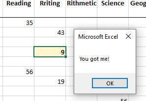
If the message isn’t appearing then you know the function isn’t working. Most likely the code is not in the correct worksheet.
Applies to
Check the Applies to conditional formatting and that you’re looking at the right part of the workbook.
Show formatting rules for: make sure it’s This worksheet or This Table.
Applies to: check the correct range is selected.
Fast Fill Sequential lists or rows in Excel
Excel Conditional Formatting, beyond the pre-sets
Text and formatting tricks for Excel
Justify, Fill, Orientation, Shrink to Fit and other Excel formatting tricks.