Use Excel with visual indicators to make lists easier to understand. Use IF function together with Conditional Formatting to display icons, text based on specific conditions
There are so many possibilities available using Conditional Formatting or simple IF statements like these.
Use IF Formula to show icons
First, decide the conditions under which icons should appear. Suppose you have a Region wise sales data in Column B and want to display icons in Column C based on sales performance:
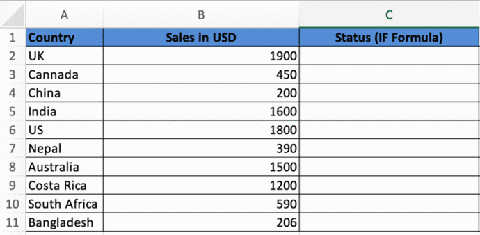
If sales are above 800, show a ✅ (Green Check) If sales are between 800 and 300, show a ⚠️ (Yellow Warning) and If sales are below 300, show a ❌ (Red Cross).
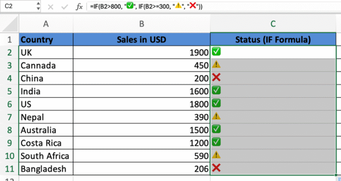
Note: they show as black icon in Excel for Windows.
Use this formula in Column C to display icons emoji based on your condition:
=IF(B2>800, “✅“, IF(B2>=300, “⚠️“, “❌“))
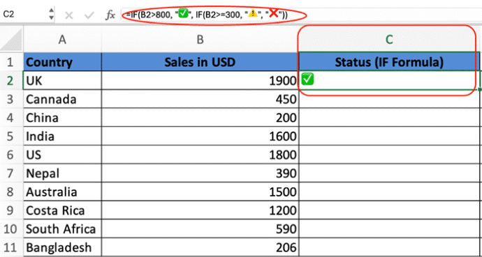
Once you see the green check icon in a cell in column C2, simply drag it down from C2 to C11 with your mouse to display the icons based on your conditions.
Use Conditional Formatting with Icon Sets
Suppose you prefer Excel’s built-in icon sets instead of text-based icons, follow these steps:
Select the cells where you want icons (e.g., C2:C11)
Navigate to Home | Conditional Formatting | Icon Sets
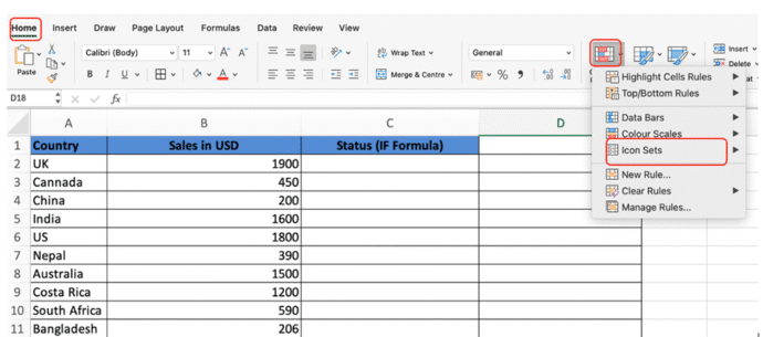
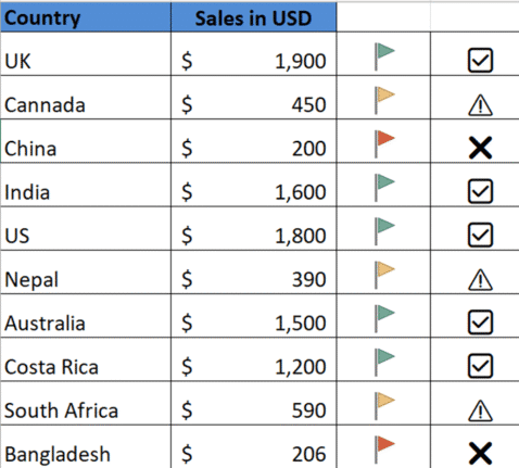
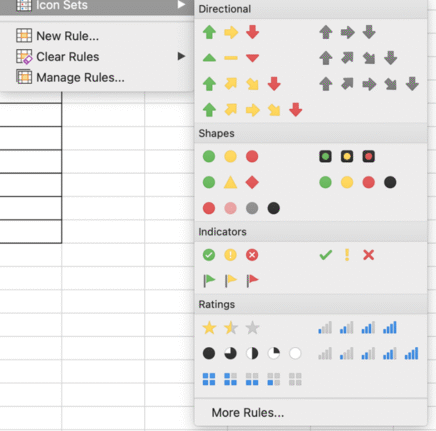
Choose an icon style from the icon sets (e.g., traffic lights, arrows, flags, etc.). Let’s choose the flag icon.
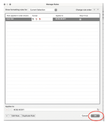
Next go to Conditional formatting |Manage Rules | Edit Rule
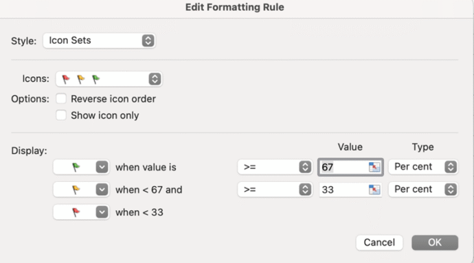
Change the type from Percent to Number and set thresholds:
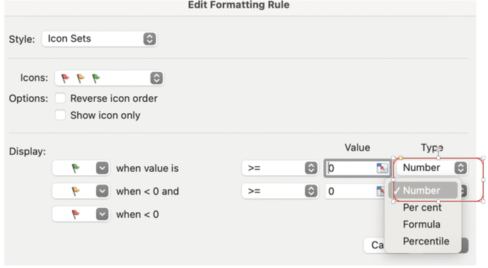
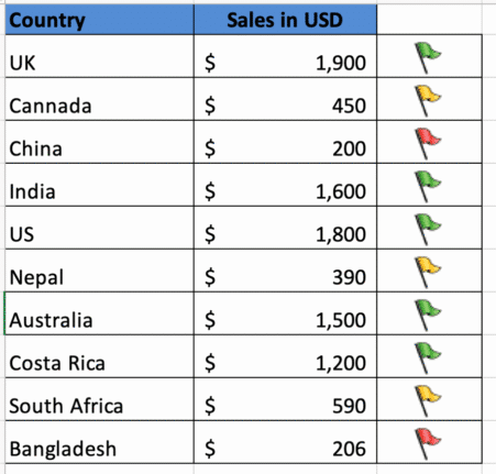
Let’s say green flag for values >1000, Yellow flag for values >300 and Red flag for values <300.
Select the “Show Icon Only” checkbox to display icons instead of numbers, based on your preference.
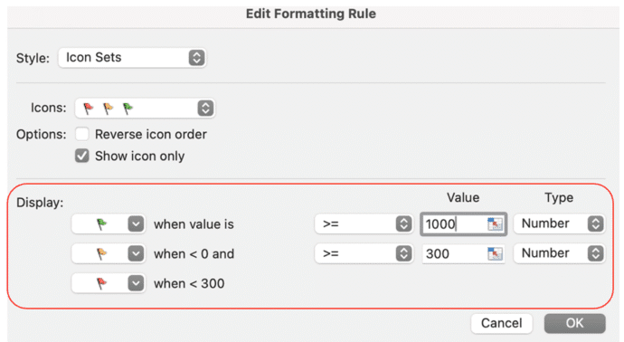
Click OK to apply.
Now, your column will display icons dynamically based on the conditional formatting.
IF and Nested IF Statements in Excel