If you have two lists in Excel and need to know what they share or where they differ, you are in the right place. Whether you are cross-checking a customer list against an invoice log, comparing a product catalog to a stock count, or reconciling two batches of data, Excel has a handful of formulas handle the job cleanly and automatically. This guide shows you exactly how to use COUNTIF with FILTER to find matches, spot missing items, and keep your results updating live as your data changes. For all Excel versions, with the best results in Excel 365, Excel 2024, and Excel 2021.
You have two lists in Excel and you want to know what they have in common or what’s missing from one of them. Maybe it’s a customer list versus an invoice list, a product catalog versus a stock count, or two batches of survey responses.
Excel has no built-in “compare these columns” button, but some straightforward formulas handles thesecommon tasks:
- Listing matches or common elements in both columns
- What’s in Column A not in Column B.
- What’s in Column B not in Column A.
This can be done in any Excel version but it’s best in Excel 365, Excel 2024/2021 and Excel on the web because they have the Filter() function. We also have formulas for Excel 2019 and before.
Here’s our example comparing a list of dwarf names proposed vs actually used in the 1937 Disney classic Snow White and the Seven Dwarfs.

Putting the lists in a table makes the formulas more readable.
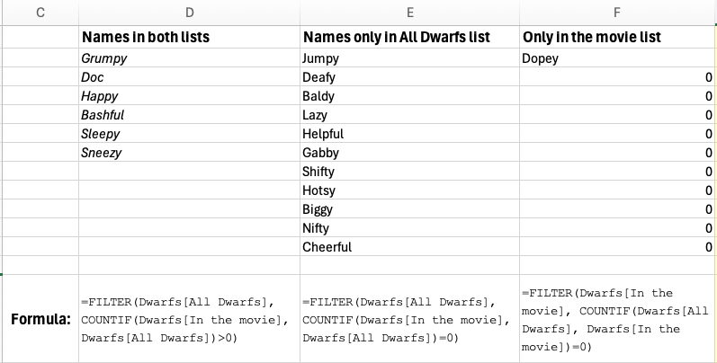
Here’s the above columns rearranged in three ways.
The key ingredient: COUNTIF
All the formulas here rely on COUNTIF, which asks a simple question: “how many times does this value appear in that range?” If the answer is greater than zero, the value exists in both columns. If the answer is zero, it only exists in one.
That one idea powers everything below.
Find values that appear in both columns
This gives you the intersection — the values that appear in column A and column B.
Modern Excel (Microsoft 365 or Excel 2024/2021):
=FILTER(A2:A100, COUNTIF(B2:B100, A2:A100)>0)=FILTER(Dwarfs[All Dwarfs], COUNTIF(Dwarfs[In the movie], Dwarfs[All Dwarfs])>0)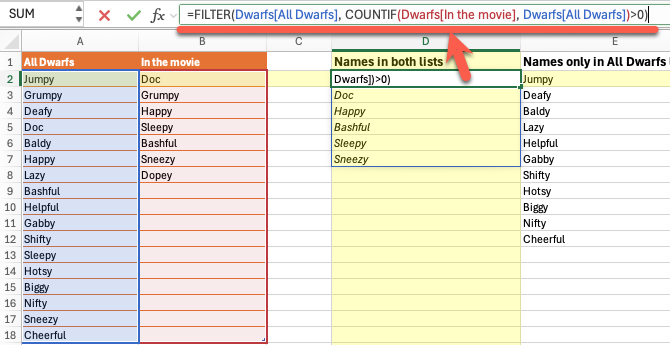
Type this in any empty cell in a third column. Excel automatically spills the results downward — no dragging, no copying. Every value from column A that also appears in column B shows up in the list.
Older Excel (2019, 2016, or earlier):
FILTER is not available in older versions. Use this in a helper column and drag it down:
=IF(COUNTIF($B$2:$B$100, A2)>0, A2, "")You will get blanks where there is no match. Sort or filter the helper column afterward to bring the matches together.
Find values in column A that are NOT in column B
Now we’ll find values that exist in column A but not from column B.
That’s remarkably easy because it’s almost the same formula as above.
Flip the comparison from >0 to =0 and you get the opposite result
Modern Excel:
=FILTER(A2:A100, COUNTIF(B2:B100, A2:A100)=0)=FILTER(Dwarfs[All Dwarfs], COUNTIF(Dwarfs[In the movie], Dwarfs[All Dwarfs])=0)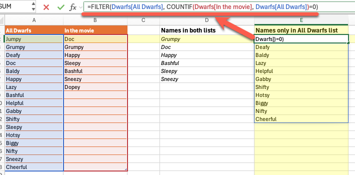
Older Excel:
=IF(COUNTIF($B$2:$B$100, A2)=0, A2, "")Same idea, same approach, just the opposite result.
Find values in column B that are NOT in column A
Now we’ll do the reverse, find values that exist in column B but not from column A.
We deliberately dropped “Dopey” from the All Dwarfs column so this demo will work!
Similar to the above formula except that the parameters are switched around.
Modern Excel:
=FILTER(Dwarfs[In the movie], COUNTIF(Dwarfs[All Dwarfs], Dwarfs[In the movie])=0)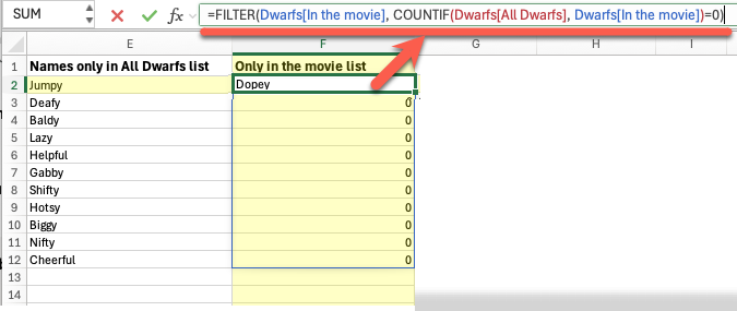
Older Excel:
=IF(COUNTIF($A:$A, B2)=0, B2, "")Automatic updates
A big advantage of dynamic array formulas like Filter() is they automatically update.
Any changes to the source lists will immediately show in the other columns.
Check for duplicates in the results
If a value appears multiple times in column A, FILTER returns it multiple times. If you want each value listed only once, wrap the formula in UNIQUE:
=UNIQUE(FILTER(A2:A100, COUNTIF(B2:B100, A2:A100)>0))UNIQUE is also a modern Excel feature (Microsoft 365 and Excel 2021). It is not available in older versions.
Sorting the results
In Excel 365, 2021 and the web, there’s a Sort() function which makes it easy to reorder a list.
Just wrap the Filter() formula with Sort()
=SORT(FILTER(Dwarfs[All Dwarfs], COUNTIF(Dwarfs[In the movie], Dwarfs[All Dwarfs])=0))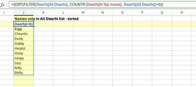
Adjust for your actual data range
The formulas above use A2:A100 and B2:B100 as placeholders. Replace those with your actual ranges.
It’s better to put the lists in an Excel Table, you can use the column names directly, which is cleaner and adjusts automatically as your table grows:
=FILTER(Dwarfs[All Dwarfs], COUNTIF(Dwarfs[In the movie], Dwarfs[All Dwarfs])>0)Easy and Better Lists with Excel 365’s Filter()
Unique() Makes a Once-Difficult Task Really Easy in Excel
Extend UNIQUE() for Distinct Values That Appear More Than Once
Three Ways to Make an Auto-Update Unique List in Excel
Excel Now Has Dynamic Arrays – Windows, Mac and More
Quick Excel List Sorting and Filter Buttons